©2011 O’Reilly Media, Inc. O’Reilly logo is a registered trademark of O’Reilly Media, Inc.
Learn how to turn
data into decisions.
From startups to the Fortune 500,
smart companies are betting on
data-driven insight, seizing the
opportunities that are emerging
from the convergence of four
powerful trends:
n New methods of collecting, managing, and analyzing data
n Cloud computing that offers inexpensive storage and flexible, on-demand computing power for massive data sets
n Visualization techniques that turn complex data into images that tell a compelling story
n Tools that make the power of data available to anyone
Get control over big data and turn it into insight with O’Reilly’s Strata offerings. Find the inspiration and information to create new products or revive existing ones, understand customer behavior, and get the data edge.
Visit oreilly.com/data to learn more.
Learning R
by Richard Cotton
Copyright © 2013 Richard Cotton. All rights reserved.
Printed in the United States of America.
Published by O’Reilly Media, Inc., 1005 Gravenstein Highway North, Sebastopol, CA 95472.
O’Reilly books may be purchased for educational, business, or sales promotional use. Online editions are also available for most titles (http://my.safaribooksonline.com). For more information, contact our corporate/ institutional sales department: 800-998-9938 or [email protected].
Editor: Meghan Blanchette Production Editor: Kristen Brown Copyeditor: Rachel Head Proofreader: Jilly Gagnon
Indexer: WordCo Indexing Services Cover Designer: Karen Montgomery Interior Designer: David Futato Illustrator: Rebecca Demarest
September 2013: First Edition
Revision History for the First Edition: 2013-09-06: First release
See http://oreilly.com/catalog/errata.csp?isbn=9781449357108 for release details.
Nutshell Handbook, the Nutshell Handbook logo, and the O’Reilly logo are registered trademarks of O’Reilly Media, Inc. Learning R, the image of a roe deer, and related trade dress are trademarks of O’Reilly Media, Inc.
Many of the designations used by manufacturers and sellers to distinguish their products are claimed as trademarks. Where those designations appear in this book, and O’Reilly Media, Inc., was aware of a trade‐ mark claim, the designations have been printed in caps or initial caps.
While every precaution has been taken in the preparation of this book, the publisher and authors assume no responsibility for errors or omissions, or for damages resulting from the use of the information contained herein.
ISBN: 978-1-449-35710-8
Table of Contents
Preface. . . xiii
Part I. The R Language
1. Introduction. . . 3
Chapter Goals 3
What Is R? 3
Installing R 4
Choosing an IDE 5
Emacs + ESS 5
Eclipse/Architect 6
RStudio 6
Revolution-R 7
Live-R 7
Other IDEs and Editors 7
Your First Program 8
How to Get Help in R 8
Installing Extra Related Software 11
Summary 11
Test Your Knowledge: Quiz 12
Test Your Knowledge: Exercises 12
2. A Scientific Calculator. . . 13
Chapter Goals 13
Mathematical Operations and Vectors 13
Assigning Variables 17
Special Numbers 19
Logical Vectors 20
Summary 22
Chapter Goals 153
Test Your Knowledge: Exercises 282
16. Programming. . . 285
Chapter Goals 285
Messages, Warnings, and Errors 286
Error Handling 289
Debugging 292
Testing 294
RUnit 295
testthat 298
Magic 299
Turning Strings into Code 299
Turning Code into Strings 301
Object-Oriented Programming 302
S3 Classes 303
Reference Classes 305
Summary 310
Test Your Knowledge: Quiz 310
Test Your Knowledge: Exercises 311
17. Making Packages. . . 313
Chapter Goals 313
Why Create Packages? 313
Prerequisites 313
The Package Directory Structure 314
Your First Package 315
Documenting Packages 317
Checking and Building Packages 320
Maintaining Packages 321
Summary 323
Test Your Knowledge: Quiz 323
Test Your Knowledge: Exercises 324
Part III. Appendixes
A. Properties of Variables. . . 327
B. Other Things to Do in R. . . 331
C. Answers to Quizzes. . . 333
D. Solutions to Exercises. . . 341
Bibliography. . . 365
Index. . . 367
Preface
R is a programming language and a software environment for data analysis and statistics. It is a GNU project, which means that it is free, open source software. It is growing exponentially by most measures—most estimates count over a million users, and it has over 4,000 add-on packages contributed by the community, with that number increasing by about 25% each year. The Tiobe Programming Community Index of language pop‐ ularity places it at number 24 at the time of this writing, roughly on a par with SAS and MATLAB.
R is used in almost every area where statistics or data analyses are needed. Finance, marketing, pharmaceuticals, genomics, epidemiology, social sciences, and teaching are all covered, as well as dozens of other smaller domains.
About This Book
Since R is primarily designed to let you do statistical analyses, many of the books written about R focus on teaching you how to calculate statistics or model datasets. This un‐ fortunately misses a large part of the reality of analyzing data. Unless you are doing cutting-edge research, the statistical techniques that you use will often be routine, and the modeling part of your task may not be the largest one. The complete workflow for analyzing data looks more like this:
1. Retrieve some data. 2. Clean the data.
3. Explore and visualize the data. 4. Model the data and make predictions. 5. Present or publish your results.
Of course at each stage your results may generate interesting questions that lead you to look for more data, or for a different way to treat your existing data, which can send you back a step. The workflow can be iterative, but each of the steps needs to be undertaken.
The first part of this book is designed to teach you R from scratch—you don’t need any experience in the language. In fact, no programming experience at all is necessary, but if you have some basic programming knowledge, it will help. For example, the book explains how to comment your code and how to write a for loop, but doesn’t explain in great detail what they are. If you want a really introductory text on how to program, then Python for Kids by Jason R. Briggs is as good a place to start as any!
The second part of the book takes you through the complete data analysis workflow in R. Here, some basic statistical knowledge is assumed. For example, you should under‐ stand terms like mean and standard deviation, and what a bar chart is.
The book finishes with some more advanced R topics, like object-oriented program‐ ming and package creation. Garrett Grolemund’s Data Analysis with R picks up where this book leaves off, covering data analysis workflow in more detail.
A word of warning: this isn’t a reference book, and many of the topics aren’t covered in great detail. This book provides tutorials to give you ideas about what you can do in R and let you practice. There isn’t enough room to cover all 4,000 add-on packages, but by the time you’ve finished reading, you should be able to find the ones that you need, and get the help you need to start using them.
What Is in This Book
This is a book of two halves. The first half is designed to provide you with the technical skills you need to use R; each chapter is a short introduction to a different set of data types (for example, Chapter 4 covers vectors, matrices, and arrays) or a concept (for example, Chapter 8 covers branching and looping).
The second half of the book ramps up the fun: you get to see real data analysis in action. Each chapter covers a section of the standard data analysis workflow, from importing data to publishing your results.
Here’s what you’ll find in Part I, The R Language:
• Chapter 1, Introduction, tells you how to install R and where to get help.
• Chapter 2, A Scientific Calculator, shows you how to use R as a scientific calculator. • Chapter 3, Inspecting Variables and Your Workspace, lets you inspect variables in
different ways.
• Chapter 4, Vectors, Matrices, and Arrays, covers vectors, matrices, and arrays.
• Chapter 5, Lists and Data Frames, covers lists and data frames (for spreadsheet-like data).
• Chapter 6, Environments and Functions, covers environments and functions. • Chapter 7, Strings and Factors, covers strings and factors (for categorical data). • Chapter 8, Flow Control and Loops, covers branching (if and else), and basic
looping.
• Chapter 9, Advanced Looping, covers advanced looping with the apply function and its variants.
• Chapter 10, Packages, explains how to install and use add-on packages. • Chapter 11, Dates and Times, covers dates and times.
Here are the topics covered in Part II, The Data Analysis Workflow:
• Chapter 12, Getting Data, shows you how to import data into R.
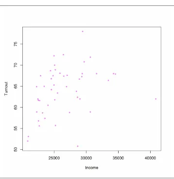
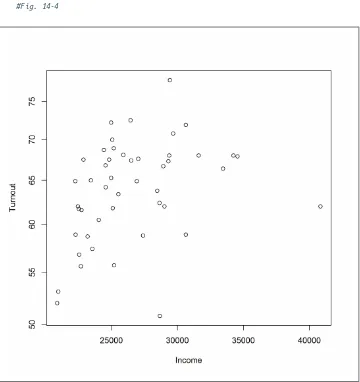
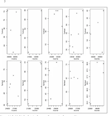
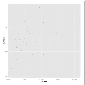
• Chapter 13, Cleaning and Transforming, explains cleaning and manipulating data. • Chapter 14, Exploring and Visualizing, lets you explore data by calculating statistics
and plotting.
• Chapter 15, Distributions and Modeling, introduces modeling.
• Chapter 16, Programming, covers a variety of advanced programming techniques. • Chapter 17, Making Packages, shows you how to package your work for others.
Lastly, there are useful references in Part III, Appendixes:
• Appendix A, Properties of Variables, contains tables comparing the properties of different types of variables.
• Appendix B, Other Things to Do in R, describes some other things that you can do in R.
• Appendix C, Answers to Quizzes, contains the answers to the end-of-chapter quizzes.
• Appendix D, Solutions to Exercises, contains the answers to the end of chapter pro‐ gramming exercises.
Which Chapters Should I Read?
If you have never used R before, then start at the beginning and work through chapter by chapter. If you already have some experience with R, you may wish to skip the first chapter and skim the chapters on the R core language.
1. Andrie’s book covers much the same ground as Learning R, and in many ways is almost as good as this work, so I won’t be offended if you want to read it too.
Each chapter deals with a different topic, so although there is a small amount of de‐ pendency from one chapter to the next, it is possible to pick and choose chapters that interest you.
I recently discussed this matter with Andrie de Vries, author of R For Dummies. He suggested giving up and reading his book instead!1
Conventions Used in This Book
The following font conventions are used in this book:
Italic
Indicates new terms, URLs, email addresses, file and pathnames, and file extensions.
Constant width
Used for code samples that should be copied verbatim, as well as within paragraphs to refer to program elements such as variable or function names, data types, envi‐ ronment variables, statements, and keywords. Output from blocks of code is also in constant width, preceded by a double hash (##).
Constant width italic
Shows text that should be replaced with user-supplied values or by values deter‐ mined by context.
There is a style guide for the code used in this book at http://4dpiecharts.com/r-code-style-guide.
This icon signifies a tip, suggestion, or general note.
This icon indicates a warning or caution.
Goals, Summaries, Quizzes, and Exercises
Each chapter begins with a list of goals to let you know what to expect in the forthcoming pages, and finishes with a summary that reiterates what you’ve learned. You also get a quiz, to make sure you’ve been concentrating (and not just pretending to read while watching telly). The answers to the questions can be found within the chapter (or at the
end of the book, if you want to cheat). Finally, each chapter concludes with some exer‐ cises, most of which involve you writing some R code. After each exercise description there is a number in square brackets, denoting a generous estimate of how many minutes it might take you to complete it.
Using Code Examples
Supplemental material (code examples, exercises, etc.) is available for download at http://cran.r-project.org/web/packages/learningr.
This book is here to help you get your job done. In general, if example code is offered with this book, you may use it in your programs and documentation. You do not need to contact us for permission unless you’re reproducing a significant portion of the code. For example, writing a program that uses several chunks of code from this book does not require permission. Selling or distributing a CD-ROM of examples from O’Reilly books does require permission. Answering a question by citing this book and quoting example code does not require permission. Incorporating a significant amount of ex‐ ample code from this book into your product’s documentation does require permission.
We appreciate, but do not require, attribution. An attribution usually includes the title, author, publisher, and ISBN. For example: "Learning R by Richard Cotton (O’Reilly). Copyright 2013 Richard Cotton, 978-1-449-35710-8.”
If you feel your use of code examples falls outside fair use or the permission given above, feel free to contact us at [email protected].
Safari® Books Online
Safari Books Online is an on-demand digital library that delivers expert content in both book and video form from the world’s lead‐ ing authors in technology and business.
Technology professionals, software developers, web designers, and business and crea‐ tive professionals use Safari Books Online as their primary resource for research, prob‐ lem solving, learning, and certification training.
Safari Books Online offers a range of product mixes and pricing programs for organi‐ zations, government agencies, and individuals. Subscribers have access to thousands of books, training videos, and prepublication manuscripts in one fully searchable database from publishers like O’Reilly Media, Prentice Hall Professional, Addison-Wesley Pro‐ fessional, Microsoft Press, Sams, Que, Peachpit Press, Focal Press, Cisco Press, John Wiley & Sons, Syngress, Morgan Kaufmann, IBM Redbooks, Packt, Adobe Press, FT Press, Apress, Manning, New Riders, McGraw-Hill, Jones & Bartlett, Course Technol‐ ogy, and dozens more. For more information about Safari Books Online, please visit us online.
How to Contact Us
Please address comments and questions concerning this book to the publisher:
O’Reilly Media, Inc.
1005 Gravenstein Highway North Sebastopol, CA 95472
800-998-9938 (in the United States or Canada) 707-829-0515 (international or local)
707-829-0104 (fax)
We have a web page for this book, where we list errata, examples, and any additional information. You can access this page at http://oreil.ly/learningR.
To comment or ask technical questions about this book, send email to bookques [email protected].
For more information about our books, courses, conferences, and news, see our website at http://www.oreilly.com.
Find us on Facebook: http://facebook.com/oreilly
Follow us on Twitter: http://twitter.com/oreillymedia
Watch us on YouTube: http://www.youtube.com/oreillymedia
Acknowledgments
Many amazing people have helped with the making of this book, not least my excellent editor Meghan Blanchette, who is full of sensible advice.
Data was donated by several wonderful people:
• Bill Hogan of AMD found and cleaned the Alpe d’Huez cycling dataset, and pointed me toward the CDC gonorrhoea dataset. He wanted me to emphasize that he’s disease-free, ladies.
• Ewan Hunter of CEFAS provided the North Sea crab dataset.
• Corina Logan of the University of Cambridge compiled and provided the deer skull data.
• Edwin Thoen of Leiden University compiled and provided the Obama vs. McCain dataset.
• Gwern Branwen compiled the hafu dataset by watching and reading an inordinate amount of manga. Kudos.
Many other people sent me datasets; there wasn’t room for them all, but thank you anyway!
Bill Hogan also reviewed the book, as did Daisy Vincent of Marin Software, and JD Long. I don’t know where JD works, but he lives in Bermuda, so it probably involves triangles. Additional comments and feedback were provided by James White, Ben Hanks, Beccy Smith, and Guy Bourne of TDX Group; Alex Hogg and Adrian Kelsey of HSL; Tom Hull, Karen Vanstaen, Rachel Beckett, Georgina Rimmer, Ruth Wortham, Bernardo Garcia-Carreras, and Joana Silva of CEFAS; Tal Galili of Tel Aviv University; Garrett Grolemund of RStudio; and John Verzani of the City University of New York. David Maxwell of CEFAS wonderfully recruited more or less everyone else in CEFAS to review my book.
John Verzani also deserves much credit for helping conceive this book, and for providing advice on the structure.
Sanders Kleinfeld of O’Reilly provided great tech support when I was pulling my hair out over character encodings in the manuscript. Yihui Xie went above and beyond the call of duty helping me get knitr to generate AsciiDoc. Rachel Head single-handedly spotted over 4,000 bugs, typos, and mistakes while copyediting.
Garib Murshudov was the lecturer who first taught me R, back in 2004.
Finally, Janette Bowler deserves a medal for her endless patience and support while I’ve been busy writing.
CHAPTER 1
Introduction
Congratulations! You’ve just begun your quest to become an R programmer. So you don’t pull any mental muscles, this chapter starts you off gently with a nice warm-up. Before you begin coding, we’re going to talk about what R is, and how to install it and begin working with it. Then you’ll try writing your first program and learn how to get help.
Chapter Goals
After reading this chapter, you should:
• Know some things that you can use R to do • Know how to install R and an IDE to work with it • Be able to write a simple program in R
• Know how to get help in R
What Is R?
Just to confuse you, R refers to two things. There is R, the programming language, and R, the piece of software that you use to run programs written in R. Fortunately, most of the time it should be clear from the context which R is being referred to.
R (the language) was created in the early 1990s by Ross Ihaka and Robert Gentleman, then both working at the University of Auckland. It is based upon the S language that was developed at Bell Laboratories in the 1970s, primarily by John Chambers. R (the software) is a GNU project, reflecting its status as important free and open source soft‐ ware. Both the language and the software are now developed by a group of (currently) 20 people known as the R Core Team.
1. Intelligently designed?
2. A look in the Internet Archive’s Wayback Machine suggests that the front page hasn’t changed much since May 2004.
The fact that R’s history dates back to the 1970s is important, because it has evolved over the decades, rather than having been designed from scratch (contrast this with, for example, Microsoft’s .NET Framework, which has a much more “created”1 feel). As with life-forms, the process of evolution has led to some quirks and inconsistencies. The upside of the more free-form nature of R (and the free license in particular) is that if you don’t like how something in R is done, you can write a package to make it do things the way that you want. Many people have already done that, and the common question now is not “Can I do this in R?” but “Which of the three implementations should I use?”
R is an interpreted language (sometimes called a scripting language), which means that your code doesn’t need to be compiled before you run it. It is a high-level language in that you don’t have access to the inner workings of the computer you are running your code on; everything is pitched toward helping you analyze data.
R supports a mixture of programming paradigms. At its core, it is an imperative language (you write a script that does one calculation after another), but it also supports object-oriented programming (data and functions are combined inside classes) and functional programming (functions are first-class objects; you treat them like any other variable, and you can call them recursively). This mix of programming styles means that R code can bear a lot of similarity to several other languages. The curly braces mean that you can write imperative code that looks like C (but the vectorized nature of R that we’ll discuss in Chapter 2 means that you have fewer loops). If you use reference classes, then you can write object-oriented code that looks a bit like C# or Java. The functional pro‐ gramming constructs are Lisp-inspired (the variable-scoping rules are taken from the Lisp dialect, Scheme), but there are fewer brackets. All this is a roundabout way of saying that R follows the Perl ethos:
There is more than one way to do it.
— Larry Wall
Installing R
If you are using a Linux machine, then it is likely that your package manager will have R available, though possibly not the latest version. For everyone else, to install R you must first go to http://www.r-project.org. Don’t be deceived by the slightly archaic web‐ site;2 it doesn’t reflect on the quality of R. Click the link that says “download R” in the “Getting Started” pane at the bottom of the page.
3. You don’t need to limit yourself to just one way of using R. I have IDE commitment issues and use a mix of Eclipse + StatET, RStudio, Live-R, Tinn-R, Notepad++, and R GUI. Experiment, and find something that works for you.
Once you’ve chosen a mirror close to you, choose a link in the “Download and Install R” pane at the top of the page that’s appropriate to your operating system. After that there are one or two OS-specific clicks that you need to make to get to the download.
If you are a Windows user who doesn’t like clicking, there is a cheeky shortcut to the setup file at http://<CRAN MIRROR>/bin/windows/base/release.htm.
Choosing an IDE
If you use R under Windows or Mac OS X, then a graphical user interface (GUI) is available to you. This consists of a command-line interpreter, facilities for displaying plots and help pages, and a basic text editor. It is perfectly possible to use R in this way, but for serious coding you’ll at least want to use a more powerful text editor. There are countless text editors for programmers; if you already have a favorite, then take a look to see if you can get syntax highlighting of R code for it.
If you aren’t already wedded to a particular editor, then I suggest that you’ll get the best experience of R by using an integrated development environment (IDE). Using an IDE rather than a separate text editor gives you the benefit of only using one piece of software rather than two. You get all the facilities of the stock R GUI, but with a better editor, and in some cases things like integrated version control.
The following sections introduce five popular choices, but this is by no means an ex‐ haustive list (a few additional suggestions follow). It is worth trying several IDEs; a development environment is a piece of software that you could be spending thousands of hours using, so it’s worth taking the time to find one3 that you like. A few additional suggestions follow this selection.
Emacs + ESS
Although Emacs calls itself a text editor, 36 years (and counting) of development have given it an unparalleled number of features. If you’ve been programming for any sub‐ stantial length of time, you probably already know whether or not you want to use it. Converts swear by its limitless customizability and raw editing power; others complain that it overcomplicates things and that the key chords give them repetitive strain injury. There is certainly a steep learning curve, so be willing to spend a month or two getting used to it. The other big benefit is that Emacs is not R-specific, so you can use it for programming in many languages. The original version of Emacs is (like R) a GNU project, available from http://www.gnu.org/software/emacs/.
Another popular fork is XEmacs, available from http://www.xemacs.org/.
Emacs Speaks Statistics (ESS) is an add-on for Emacs that assists you in writing R code. Actually, it works with S-Plus, SAS, and Stata, too, so you can write statistical code with whichever package you like (choose R!). Several of the authors of ESS are also R Core Team members, so you are guaranteed good integration with R. It is available through the Emacs package management system, or you can download it from http://ess.r-project.org/.
Use it if you want to write code in multiple languages, you want the most powerful editor available, and you are fearless with learning curves.
Eclipse/Architect
Eclipse is another cross-platform IDE, widely used in the Java community. Like Emacs, it is very powerful, and its plug-in system makes it highly customizable. The learning curve is shallower, though, and it allows for more pointing and clicking than the heavily keyboard-driven Emacs.
Architect is an R-oriented variant of Eclipse developed by statistics consultancy Open Analytics. It includes the StatET plug-in for integration with R, including a debugger that is superior to the one built into R GUI. Download it from http://www.openanalyt ics.eu/downloads/architect.
Alternatively, you can get the standard Eclipse IDE from http://eclipse.org and use its package manager to download the StatET plug-in from http://www.walware.de/goto/ statet.
Use it if you want to write code in multiple languages, you don’t have time to learn Emacs, and you don’t mind a several-hundred-megabyte install.
RStudio
RStudio is an R-specific IDE. That means that you lose the ability to code (easily) in multiple languages, but you do get some features especially for R. For example, the plot windows are better than the R GUI originals, and there are facilities for publishing code. The editor is more basic than either Emacs or Eclipse, but it’s good enough for most purposes, and is easier to get started with than the other two. RStudio’s party trick is that you can run it remotely through a browser, so you can run R on a powerful server, then access it from a netbook (or smartphone) without loss of computational power. Download it from http://www.rstudio.org.
Use it if you mainly write R code, don’t need advanced editor features, and want a shallow learning curve or the ability to run remotely.
Revolution-R
Revolution-R comes in two flavors: the free (as in beer) community edition and the paid-for enterprise edition. Both take a different tack from the other IDEs mentioned so far: whereas Emacs, Eclipse, and RStudio are pure graphical frontends that let you connect to any version of R, Revolution-R ships with its own customized version of R. Typically this is a stable release, one or two versions back from the most current. It also has some enhancements for working with big data, and some enterprise-related features. Download it from http://www.revolutionanalytics.com/products/revolution-r.php.
Use it if you mainly write R code, you work with big data or want a paid support contract, or you require extra stability in your R platform.
Live-R
Live-R is a new player, in invite-only beta at the time this book is going to press. It provides an IDE for R as a web application. This avoids all the hassle of installing soft‐ ware on your machine and, like RStudio’s remote installation, gives you the ability to run R calculations from an underpowered machine. Live-R also includes a number of features for collaboration, including a shared editor and code publishing, as well as some admin tools for running courses based upon R. The main downside is that not all the add-on packages for R are available; you are currently limited to about 200 or so that are compatible with the web application. Sign up at http://live-analytics.com/.
Use it if you mainly write R code, don’t want to install any software, or want to teach a class based upon R.
Other IDEs and Editors
There are many more editors that you can use to write R code. Here’s a quick roundup of a few more possibilities:
• JGR [pronounced “Jaguar”] is a Java-based GUI for R, essentially a souped-up ver‐ sion of the stock R GUI.
• Tinn-R is a fork of the editor TINN that has extensions specifically to help you write R code.
• SciViews-K, from the same team that makes Tinn-R, is an extension for the Komodo IDE to work with R.
• Vim-R is a plug-in for Vim that provides R integration. • NppToR plugs into Notepad++ to give R integration.
Your First Program
It is a law of programming books that the first example shall be a program to print the phrase “Hello world!” In R that’s really boring, since you just type “Hello world!” at the command prompt, and it will parrot it back to you. Instead, we’re going to write the simplest statistical program possible.
Open up R GUI, or whichever IDE you’ve decided to use, find the command prompt (in the code editor window), and type:
mean(1:5)
Hit Enter to run the line of code. Hopefully, you’ll get the answer 3. As you might have guessed, this code is calculating the arithmetic mean of the numbers from 1 to 5. The colon operator, :, creates a sequence of numbers from the first number, in this case 1, to the second number (5), each separated by 1. The resulting sequence is called a vector.
mean is a function (that calculates the arithmetic mean), and the vector that we enclose inside the parentheses is called an argument to the function.
Well done! You’ve calculated a statistic using R.
In R GUI and most of the IDEs mentioned here, you can press the up arrow key to cycle back through previous commands.
How to Get Help in R
Before you get started writing R code, the most important thing to know is how to get help. There are lots of ways to do this. Firstly, if you want help on a function or a dataset that you know the name of, type ? followed by the name of the function. To find func‐ tions, type two question marks (??) followed by a keyword related to the problem to search. Special characters, reserved words, and multiword search terms need enclosing in double or single quotes. For example:
?mean #opens the help page for the mean function
?"+" #opens the help page for addition
?"if" #opens the help page for if, used for branching code
??plotting #searches for topics containing words like "plotting"
??"regression model" #searches for topics containing phrases like this
That # symbol denotes a comment. It means that R will ignore the rest of the line. Use comments to document your code, so that you can remember what you were doing six months ago.
4. apropos is Latin for “A Unix program that finds manpages.”
The functions help and help.search do the same things as ? and ??, respectively, but with these you always need to enclose your arguments in quotes. The following com‐ mands are equivalent to the previous lot:
help("mean")
help("+")
help("if")
help.search("plotting")
help.search("regression model")
The apropos function4 finds variables (including functions) that match its input. This is really useful if you can only half-remember the name of a variable that you’ve created, or a function that you want to use. For example, suppose you create a variable a_vector:
a_vector <- c(1, 3, 6, 10)
You can then recall this variable using apropos:
apropos("vector")
## [1] ".__C__vector" "a_vector" "as.data.frame.vector" ## [4] "as.vector" "as.vector.factor" "is.vector"
## [7] "vector" "Vectorize"
The results contain the variable you just created, a_vector, and all other variables that contain the string vector. In this case, all the others are functions that are built into R. Just finding variables that contain a particular string is fine, but you can also do fancier matching with apropos using regular expressions.
Regular expressions are a cross-language syntax for matching strings. The details will only be touched upon in this book, but you need to learn to use them; they’ll change your life. Start at http:// www.regular-expressions.info/quickstart.html, and then try Mi‐ chael Fitzgerald’s Introducing Regular Expressions.
A simple usage of apropos could, for example, find all variables that end in z, or to find all variables containing a number between 4 and 9:
apropos("z$")
## [1] "alpe_d_huez" "alpe_d_huez" "force_tz" "indexTZ" "SSgompertz" ## [6] "toeplitz" "tz" "unz" "with_tz"
apropos("[4-9]")
## [1] ".__C__S4" ".__T__xmlToS4:XML" ".parseISO8601" ## [4] ".SQL92Keywords" ".TAOCP1997init" "asS4"
## [7] "assert_is_64_bit_os" "assert_is_S4" "base64" ## [10] "base64Decode" "base64Encode" "blues9"
Most functions have examples that you can run to get a better idea of how they work. Use the example function to run these. There are also some longer demonstrations of concepts that are accessible with the demo function:
example(plot)
demo() #list all demonstrations
demo(Japanese)
R is modular and is split into packages (more on this later), some of which contain
vignettes, which are short documents on how to use the packages. You can browse all the vignettes on your machine using browseVignettes:
browseVignettes()
You can also access a specific vignette using the vignette function (but if your memory is as bad as mine, using browseVignettes combined with a page search is easier than trying to remember the name of a vignette and which package it’s in):
vignette("Sweave", package = "utils")
The help search operator ?? and browseVignettes will only find things in packages that you have installed on your machine. If you want to look in any package, you can use RSiteSearch, which runs a query at http://search.r-project.org. Multiword terms need to be wrapped in braces:
RSiteSearch("{Bayesian regression}")
Learning to help yourself is extremely important. Think of a key‐ word related to your work and try ?, ??, apropos, and RSiteSearch
with it.
There are also lots of R-related resources on the Internet that are worth trying. There are too many to list here, but start with these:
• R has a number of mailing lists with archives containing years’ worth of questions on the language. At the very least, it is worth signing up to the general-purpose list,
R-help.
• RSeek is a web search engine for R that returns functions, posts from the R mailing list archives, and blog posts.
• R-bloggers is the main R blogging community, and the best way to stay up to date with news and tips about R.
• The programming question and answer site Stack Overflow also has a vibrant R community, providing an alternative to the R-help mailing list. You also get points and badges for answering questions!
Installing Extra Related Software
There are a few other bits of software that R can use to extend its functionality. Under Linux, your package manager should be able to retrieve them. Under Windows, rather than hunting all over the Internet to track down this software, you can use the installr
add-on package to automatically install these extra pieces of software. None of this software is compulsory, so you can skip this section now if you want, but it’s worth knowing that the package exists when you come to need the additional software. In‐ stalling and loading packages is discussed in detail in Chapter 10, so don’t worry if you don’t understand the commands yet:
install.packages("installr") #download and install the package named installr
library(installr) #load the installr package
install.RStudio() #download and install the RStudio IDE
install.Rtools() #Rtools is needed for building your own packages
install.git() #git provides version control for your code
Summary
• R is a free, open source language for data analysis.
• It’s also a piece of software used to run programs written in R. • You can download R from http://www.r-project.org.
• You can write R code in any text editor, but there are several IDEs that make de‐ velopment easier.
• You can get help on a function by typing ? then its name.
• You can find useful functions by typing ?? then a search string, or by calling the
apropos function.
• There are many online resources for R.
Test Your Knowledge: Quiz
Question 1-1Which language is R an open source version of?
Question 1-2
Name at least two programming paradigms in which you can write R code.
Question 1-3
What is the command to create a vector of the numbers from 8 to 27?
Question 1-4
What is the name of the function used to search for help within R?
Question 1-5
What is the name of the function used to search for R-related help on the Internet?
Test Your Knowledge: Exercises
Exercise 1-1Visit http://www.r-project.org, download R, and install it. For extra credit, download and install one of the IDEs mentioned in “Other IDEs and Editors” on page 7. [30]
Exercise 1-2
The function sd calculates the standard deviation. Calculate the standard deviation of the numbers from 0 to 100. Hint: the answer should be about 29.3. [5]
Exercise 1-3
Watch the demonstration on mathematical symbols in plots, using demo(plot math). [5]
CHAPTER 2
A Scientific Calculator
R is at heart a supercharged scientific calculator, so it has a fairly comprehensive set of mathematical capabilities built in. This chapter will take you through the arithmetic operators, common mathematical functions, and relational operators, and show you how to assign a value to a variable.
Chapter Goals
After reading this chapter, you should:
• Be able to use R as a scientific calculator • Be able to assign a variable and view its value • Be able to use infinite and missing values
• Understand what logical vectors are and how to manipulate them
Mathematical Operations and Vectors
The + operator performs addition, but it has a special trick: as well as adding two num‐ bers together, you can use it to add two vectors. A vector is an ordered set of values. Vectors are tremendously important in statistics, since you will usually want to analyze a whole dataset rather than just one piece of data.
The colon operator, :, which you have seen already, creates a sequence from one number to the next, and the c function concatenates values, in this case to create vectors (con‐ catenate is a Latin word meaning “connect together in a chain”).
1. There are a few other name clashes: filter and Filter, find and Find, gamma and Gamma, nrow/ncol and
NROW/NCOL. This is an unfortunate side effect of R being an evolved rather than a designed language. Variable names are case sensitive in R, so we need to be a bit careful in this next example. The C function does something completely different to c:1
1:5 + 6:10 #look, no loops!
## [1] 7 9 11 13 15
c(1, 3, 6, 10, 15) + c(0, 1, 3, 6, 10)
## [1] 1 4 9 16 25
The colon operator and the c function are used almost every‐ where in R code, so it’s good to practice using them. Try creat‐ ing some vectors of your own now.
If we were writing in a language like C or Fortran, we would need to write a loop to perform addition on all the elements in these vectors. The vectorized nature of R’s ad‐ dition makes things easy, letting us avoid the loop. Vectors will be discussed more in “Logical Vectors” on page 20.
Vectorized has several meanings in R, the most common of which is that an operator or a function will act on each element of a vector without the need for you to explicitly write a loop. (This built-in implicit looping over elements is also much faster than ex‐ plicitly writing your own loop.) A second meaning of vectorization is when a function takes a vector as an input and calculates a summary statistic:
sum(1:5)
## [1] 15
median(1:5)
## [1] 3
A third, much less common case of vectorization is vectorization over arguments. This is when a function calculates a summary statistic from several of its input arguments. The sum function does this, but it is very unusual. median does not:
sum(1, 2, 3, 4, 5)
## [1] 15
median(1, 2, 3, 4, 5) #this throws an error
## Error: unused arguments (3, 4, 5)
All the arithmetic operators in R, not just plus (+), are vectorized. The following exam‐ ples demonstrate subtraction, multiplication, exponentiation, and two kinds of division, as well as remainder after division:
c(2, 3, 5, 7, 11, 13) - 2 #subtraction
## [1] 0 1 3 5 9 11
-2:2 * -2:2 #multiplication
## [1] 4 1 0 1 4
identical(2 ^ 3, 2 ** 3) #we can use ^ or ** for exponentiation
#though ^ is more common
## [1] TRUE
1:10 / 3 #floating point division
## [1] 0.3333 0.6667 1.0000 1.3333 1.6667 2.0000 2.3333 2.6667 3.0000 3.3333
1:10 %/% 3 #integer division
## [1] 0 0 1 1 1 2 2 2 3 3
1:10 %% 3 #remainder after division
## [1] 1 2 0 1 2 0 1 2 0 1
R also contains a wide selection of mathematical functions. You get trigonometry (sin,
cos, tan, and their inverses asin, acos, and atan), logarithms and exponents (log and
exp, and their variants log1p and expm1 that calculate log(1 + x) and exp(x - 1) more accurately for very small values of x), and almost any other mathematical function you can think of. The following examples provide a hint of what is on offer. Again, notice that all the functions naturally operate on vectors rather than just single values:
cos(c(0, pi / 4, pi / 2, pi)) #pi is a built-in constant
## [1] 1.000e+00 7.071e-01 6.123e-17 -1.000e+00
exp(pi * 1i) + 1 #Euler's formula
## [1] 0+1.225e-16i
factorial(7) + factorial(1) - 71 ^ 2 #5041 is a great number
## [1] 0
choose(5, 0:5)
## [1] 1 5 10 10 5 1
To compare integer values for equality, use ==. Don’t use a single = since that is used for something else, as we’ll see in a moment. Just like the arithmetic operators, == and the other relational operators are vectorized. To check for inequality, the “not equals” op‐ erator is !=. Greater than and less than are as you might expect: > and < (or >= and <=
if equality is allowed). Here are a few examples:
c(3, 4 - 1, 1 + 1 + 1) == 3 #operators are vectorized too
## [1] TRUE TRUE TRUE
1:3 != 3:1
## [1] TRUE FALSE TRUE
exp(1:5) < 100
## [1] TRUE TRUE TRUE TRUE FALSE
(1:5) ^ 2 >= 16
## [1] FALSE FALSE FALSE TRUE TRUE
Comparing nonintegers using == is problematic. All the numbers we have dealt with so far are floating point numbers. That means that they are stored in the form a * 2 ^ b, for two numbers a and b. Since this whole form has to be stored in 32 bits, the resulting number is only an approximation of what you really want. This means that rounding errors often creep into calculations, and the answers you expected can be wildly wrong. Whole books have been written on this subject; there is too much to worry about here. Since this is such a common mistake, the FAQ on R has an entry about it, and it’s a good place to start if you want to know more.
Consider these two numbers, which should be the same:
sqrt(2) ^ 2 == 2 #sqrt is the square-root function
## [1] FALSE
sqrt(2) ^ 2 - 2 #this small value is the rounding error
## [1] 4.441e-16
R also provides the function all.equal for checking equality of numbers. This provides a tolerance level (by default, about 1.5e-8), so that rounding errors less than the toler‐ ance are ignored:
all.equal(sqrt(2) ^ 2, 2)
## [1] TRUE
If the values to be compared are not the same, all.equal returns a report on the dif‐ ferences. If you require a TRUE or FALSE value, then you need to wrap the call to
all.equal in a call to isTRUE:
all.equal(sqrt(2) ^ 2, 3)
## [1] "Mean relative difference: 0.5"
isTRUE(all.equal(sqrt(2) ^ 2, 3))
## [1] FALSE
To check that two numbers are the same, don’t use ==. Instead, use the
all.equal function.
We can also use == to compare strings. In this case the comparison is case sensitive, so the strings must match exactly. It is also theoretically possible to compare strings using greater than or less than (> and <):
c(
"Can", "you", "can", "a", "can", "as",
"a", "canner", "can", "can", "a", "can?"
) == "can"
## [1] FALSE FALSE TRUE FALSE TRUE FALSE FALSE FALSE TRUE TRUE FALSE ## [12] FALSE
c("A", "B", "C", "D") < "C"
## [1] TRUE TRUE FALSE FALSE
c("a", "b", "c", "d") < "C" #your results may vary
## [1] TRUE TRUE TRUE FALSE
In practice, however, the latter approach is almost always an awful idea, since the results depend upon your locale (different cultures are full of odd sorting rules for letters; in Estonian, “z” comes between “s” and “t”). More powerful string matching functions will be discussed in “Cleaning Strings” on page 191.
The help pages ?Arithmetic, ?Trig, ?Special, and ?Comparison have more examples, and explain the gory details of what happens in edge cases. (Try 0 ^ 0 or integer division on nonintegers if you are curious.)
Assigning Variables
It’s all very well calculating things, but most of the time we want to store the results for reuse. We can assign a (local) variable using either <- or =, though for historical reasons,
<- is preferred:
x <- 1:5
y = 6:10
Now we can reuse these values in our further calculations:
x + 2 * y - 3
## [1] 10 13 16 19 22
Notice that we didn’t have to declare what types of variables x and y were going to be before we assigned them (unlike in most compiled languages). In fact, we couldn’t have declared the type, since no such concept exists in R.
Variable names can contain letters, numbers, dots, and underscores, but they can’t start with a number, or a dot followed by a number (since that looks too much like a number). Reserved words like “if ” and “for” are not allowed. In some locales, non-ASCII letters are allowed, but for code portability it is better to stick to “a” to “z” (and “A” to “Z”). The help page ?make.names gives precise details about what is and isn’t allowed.
The spaces around the assignment operators aren’t compulsory, but they help readabil‐ ity, especially with <-, so we can easily distinguish assignment from less than:
x <- 3 x < -3
x<-3 #is this assignment or less than?
We can also do global assignment using <<-. There’ll be more on what this means when we cover environments and scoping in “Environments” on page 79 in Chapter 6; for now, just think of it as creating a variable available anywhere:
x <<- exp(exp(1))
There is one more method of variable assignment, via the assign function. It is much less common than the other methods, but very occasionally it is useful to have a function syntax for assigning variables. Local (“normal”) assignment takes two arguments—the name of the variable to assign to and the value you want to give it:
assign("my_local_variable", 9 ^ 3 + 10 ^ 3)
Global assignment (like the <<- operator does) takes an extra argument:
assign("my_global_variable", 1 ^ 3 + 12 ^ 3, globalenv())
Don’t worry about the globalenv bit for now; as with scoping, it will be explained in Chapter 6.
Using the assign function makes your code less readable compared to
<-, so you should use it sparingly. It occasionally makes things easier in some advanced programming cases involving environments, but if your code is filled with calls to assign, you are probably doing some‐ thing wrong.
Also note that the assign function doesn’t check its first argument to see if it is a valid variable name: it always just creates it.
Notice that when you assign a variable, you don’t see the value that has been given to it. To see what value a variable contains, simply type its name at the command prompt to print it:
2. Since the numbers are random, expect to get different values if you try this yourself.
x
## [1] 1 2 3 4 5
Under some systems, for example running R from a Linux terminal, you may have to explicitly call the print function to see the value. In this case, type print(x).
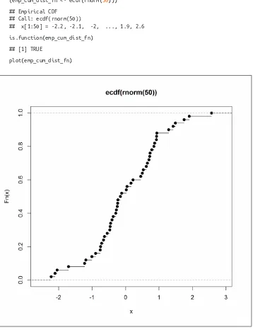
If you want to assign a value and print it all in one line, you have two possibilities. Firstly, you can put multiple statements on one line by separating them with a semicolon, ;. Secondly, you can wrap the assignment in parentheses, (). In the following examples,
rnorm generates random numbers from a normal distribution, and rlnorm generates them from a lognormal distribution:2
z <- rnorm(5); z
## [1] 1.8503 -0.5787 -1.4797 -0.1333 -0.2321
(zz <- rlnorm(5))
## [1] 1.0148 4.2476 0.3574 0.2421 0.3163
Special Numbers
To help with arithmetic, R supports four special numeric values: Inf, -Inf, NaN, and
NA. The first two are, of course, positive and negative infinity, but the second pair need a little more explanation. NaN is short for “not-a-number,” and means that our calculation either didn’t make mathematical sense or could not be performed properly. NA is short for “not available” and represents a missing value—a problem all too common in data analysis. In general, if our calculation involves a missing value, then the results will also be missing:
c(Inf + 1, Inf - 1, Inf - Inf)
## [1] Inf Inf NaN
c(1 / Inf, Inf / 1, Inf / Inf)
## [1] 0 Inf NaN
c(sqrt(Inf), sin(Inf))
## Warning: NaNs produced
## [1] Inf NaN
c(log(Inf), log(Inf, base = Inf))
## Warning: NaNs produced
## [1] Inf NaN
c(NA + 1, NA * 5, NA + Inf)
## [1] NA NA NA
When arithmetic involves NA and NaN, the answer is one of those two values, but which of those two is system dependent:
c(NA + NA, NaN + NaN, NaN + NA, NA + NaN)
## [1] NA NaN NaN NA
There are functions available to check for these special values. Notice that NaN and NA
are neither finite nor infinite, and NaN is missing but NAis a number:
x <- c(0, Inf, -Inf, NaN, NA)
is.finite(x)
## [1] TRUE FALSE FALSE FALSE FALSE
is.infinite(x)
## [1] FALSE TRUE TRUE FALSE FALSE
is.nan(x)
## [1] FALSE FALSE FALSE TRUE FALSE
is.na(x)
## [1] FALSE FALSE FALSE TRUE TRUE
Logical Vectors
In addition to numbers, scientific calculation often involves logical values, particularly as a result of using the relational operators (<, etc.). Many programming languages use Boolean logic, where the values can be either TRUE or FALSE. In R, the situation is a little bit more complicated, since we can also have missing values, NA. This three-state system is sometimes call troolean logic, although that’s a bad etymological joke, since the “Bool” in “Boolean” comes from George Bool, rather than anything to do with the word binary.
TRUE and FALSE are reserved words in R: you cannot create a variable with either of those names (lower- or mixed-case versions like True are fine, though). When you start R the variables T and F are already defined for you, taking the values TRUE and FALSE, respectively. This can save you a bit of typing, but it can also cause big problems. T and
F are not reserved words, so users can redefine them. This means that it is OK to use the abbreviated names if you are tapping away at the command line, but not if your code is going to interact with someone else’s (especially if their code involves Times or
Temperatures or mathematical Functions).
There are three vectorized logical operators in R:
## [1] FALSE FALSE FALSE FALSE FALSE TRUE FALSE TRUE FALSE TRUE
x | y
## [1] FALSE TRUE FALSE TRUE TRUE TRUE TRUE TRUE TRUE TRUE
Two other useful functions for dealing with logical vectors are any and all, which return
TRUE if the input vector contains at least one TRUE value or onlyTRUE values, respectively:
none_true <- c(FALSE, FALSE, FALSE)
some_true <- c(FALSE, TRUE, FALSE)
all_true <- c(TRUE, TRUE, TRUE)
any(none_true)
## [1] FALSE
any(some_true)
## [1] TRUE
any(all_true)
## [1] TRUE
all(none_true)
## [1] FALSE
all(some_true)
## [1] FALSE
all(all_true)
## [1] TRUE
Summary
• R can be used as a very powerful scientific calculator. • Assigning variables lets you reuse values.
• R has special values for positive and negative infinity, not-a-number, and missing values, to assist with mathematical operations.
• R uses troolean logic.
Test Your Knowledge: Quiz
Question 2-1What is the operator used for integer division?
Question 2-2
How would you check if a variable, x, is equal to pi?
Question 2-3
Describe at least two ways of assigning a variable.
Question 2-4
Which of the five numbers 0, Inf, -Inf, NaN, and NA are infinite?
Question 2-5
Which of the five numbers 0, Inf, -Inf, NaN, and NA are considered not missing?
Test Your Knowledge: Exercises
Exercise 2-1
1. Calculate the inverse tangent (a.k.a. arctan) of the reciprocal of all integers from 1 to 1,000. Hint: take a look at the ?Trig help page to find the inverse tangent function. You don’t need a function to calculate reciprocals. [5]
2. Assign the numbers 1 to 1,000 to a variable x. Calculate the inverse tangent of the reciprocal of x, as in part (a), and assign it to a variable y. Now reverse the operations by calculating the reciprocal of the tangent of y and assigning this value to a variable z. [5]
Exercise 2-2
Compare the variables x and z from Exercise 2-1 (b) using ==, identical, and
all.equal. For all.equal, try changing the tolerance level by passing a third ar‐ gument to the function. What happens if the tolerance is set to 0? [10]
Exercise 2-3
Define the following vectors:
1. true_and_missing, with the values TRUE and NA (at least one of each, in any order)
2. false_and_missing, with the values FALSE and NA
3. mixed, with the values TRUE, FALSE, and NA
Apply the functions any and all to each of your vectors. [5]
CHAPTER 3
Inspecting Variables and Your Workspace
So far, we’ve run some calculations and assigned some variables. In this chapter, we’ll find out ways to examine the properties of those variables and to manipulate the user workspace that contains them.
Chapter Goals
After reading this chapter, you should:
• Know what a class is, and the names of some common classes • Know how to convert a variable from one type to another
• Be able to inspect variables to find useful information about them • Be able to manipulate the user workspace
Classes
All variables in R have a class, which tells you what kinds of variables they are. For example, most numbers have class numeric (see the next section for the other types), and logical values have class logical. Actually, being picky about it, vectors of numbers are numeric and vectors of logical values are logical, since R has no scalar types. The “smallest” data type in R is a vector.
You can find out what the class of a variable is using class(my_variable):
class(c(TRUE, FALSE))
## [1] "logical"
It’s worth being aware that as well as a class, all variables also have an internal storage type (accessed via typeof), a mode (see mode), and a storage mode (storage.mode). If
this sounds complicated, don’t worry! Types, modes, and storage modes mostly exist for legacy purposes, so in practice you should only ever need to use an object’s class
(at least until you join the R Core Team). Appendix A has a reference table showing the relationships between class, type, and (storage) mode for many sorts of variables. Don’t bother memorizing it, and don’t worry if you don’t recognize some of the classes. It is simply worth browsing the table to see which things are related to which other things.
From now on, to make things easier, I’m going to use “class” and “type” synonymously (except where noted).
Different Types of Numbers
All the variables that we created in the previous chapter were numbers, but R contains three different classes of numeric variable: numeric for floating point values; integer
for, ahem, integers; and complex for complex numbers. We can tell which is which by examining the class of the variable:
class(sqrt(1:10))
## [1] "numeric"
class(3 + 1i) #"i" creates imaginary components of complex numbers
## [1] "complex"
class(1) #although this is a whole number, it has class numeric
## [1] "numeric"
class(1L) #add a suffix of "L" to make the number an integer
## [1] "integer"
class(0.5:4.5) #the colon operator returns a value that is numeric...
## [1] "numeric"
class(1:5) #unless all its values are whole numbers
## [1] "integer"
Note that as of the time of writing, all floating point numbers are 32-bit numbers (“dou‐ ble precision”), even when installed on a 64-bit operating system, and 16-bit (“single precision”) numbers don’t exist.
Typing .Machine gives you some information about the properties of R’s numbers. Al‐ though the values, in theory, can change from machine to machine, for most builds, most of the values are the same. Many of the values returned by .Machine need never concern you. It’s worth knowing that the largest floating point number that R can rep‐ resent at full precision is about 1.8e308. This is big enough for everyday purposes, but a lot smaller than infinity! The smallest positive number that can be represented is
1. If these limits aren’t good enough for you, higher-precision values are available via the Rmpfr package, and very large numbers are available in the brobdingnab package. These are fairly niche requirements, though; the three built-in classes of R numbers should be fine for almost all purposes.
2.2e-308. Integers can take values up to 2 ^ 31 - 1, which is a little over two billion, (or down to -2 ^ 31 + 1).1
The only other value of much interest is ε, the smallest positive floating point number such that |ε + 1| != 1. That’s a fancy way of saying how close two numbers can be so that R knows that they are different. It’s about 2.2e-16. This value is used by all.equal
when you compare two numeric vectors.
In fact, all of this is even easier than you think, since it is perfectly possible to get away with not (knowingly) using integers. R is designed so that anywhere an integer is needed —indexing a vector, for example—a floating point “numeric” number can be used just as well.
Other Common Classes
In addition to the three numeric classes and the logical class that we’ve seen already, there are three more classes of vectors: character for storing text, factors for storing categorical data, and the rarer raw for storing binary data.
In this next example, we create a character vector using the c operator, just like we did for numeric vectors. The class of a character vector is character:
class(c("she", "sells", "seashells", "on", "the", "sea", "shore"))
## [1] "character"
Note that unlike some languages, R doesn’t distinguish between whole strings and in‐ dividual characters—a string containing one character is treated the same as any other string. Unlike with some other lower-level languages, you don’t need to worry about terminating your strings with a null character (\0). In fact, it is an error to try to include such a character in your strings.
In many programming languages, categorical data would be represented by integers. For example, gender could be represented as 1 for females and 2 for males. A slightly better solution would be to treat gender as a character variable with the choices “female” and “male.” This is still semantically rather dubious, though, since categorical data is a different concept to plain old text. R has a more sophisticated solution that combines both these ideas in a semantically correct class—factors are integers with labels:
(gender <- factor(c("male", "female", "female", "male", "female")))
## [1] male female female male female ## Levels: female male
2. Or hood, if you prefer.
The contents of the factor look much like their character equivalent—you get readable labels for each value. Those labels are confined to specific values (in this case “female” and “male”) known as the levels of the factor:
levels(gender)
## [1] "female" "male"
nlevels(gender)
## [1] 2
Notice that even though “male” is the first value in gender, the first level is “female.” By default, factor levels are assigned alphabetically.
Underneath the bonnet,2 the factor values are stored as integers rather than characters. You can see this more clearly by calling as.integer:
as.integer(gender)
## [1] 2 1 1 2 1
This use of integers for storage makes them very memory-efficient compared to char‐ acter text, at least when there are lots of repeated strings, as there are here. If we exag‐ gerate the situation by generating 10,000 random genders (using the sample function to sample the strings “female” and “male” 10,000 times with replacement), we can see that a factor containing the values takes up less memory than the character equivalent. In the following code, sample returns a character vector—which we convert into a factor using as.factor--and object.size returns the memory allocation for each object:
gender_char <- sample(c("female", "male"), 10000, replace = TRUE)
gender_fac <- as.factor(gender_char)
object.size(gender_char)
## 80136 bytes
object.size(gender_fac)
## 40512 bytes
Variables take up different amounts of memory on 32-bit and 64-bit systems, so object.size will return different values in each case.
For manipulating the contents of factor levels (a common case would be cleaning up names, so all your men have the value “male” rather than “Male”) it is typically best to
3. It is unclear what a cooked byte would entail.
convert the factors to strings, in order to take advantage of string manipulation func‐ tions. You can do this in the obvious way, using as.character:
as.character(gender)
## [1] "male" "female" "female" "male" "female"
There is much more to learn about both character vectors and factors; they will be covered in depth in Chapter 7.
The raw class stores vectors of “raw” bytes.3 Each byte is represented by a two-digit hexadecimal value. They are primarily used for storing the contents of imported binary files, and as such are reasonably rare. The integers 0 to 255 can be converted to raw using
as.raw. Fractional and imaginary parts are discarded, and numbers outside this range are treated as 0. For strings, as.raw doesn’t work; you must use charToRaw instead:
as.raw(1:17)
## [1] 01 02 03 04 05 06 07 08 09 0a 0b 0c 0d 0e 0f 10 11
as.raw(c(pi, 1 + 1i, -1, 256))
## Warning: imaginary parts discarded in coercion
## Warning: out-of-range values treated as 0 in coercion to raw
## [1] 03 01 00 00
(sushi <- charToRaw("Fish!"))
## [1] 46 69 73 68 21
class(sushi)
## [1] "raw"
As well as the vector classes that we’ve seen so far, there are many other types of variables; we’ll spend the next few chapters looking at them.
Arrays contain multidimensional data, and matrices (via the matrix class) are the special case of two-dimensional arrays. They will be discussed in Chapter 4.
So far, all these variable types need to contain the same type of thing. For example, a
character vector or array must contain all strings, and a logical vector or array must contain only logical values. Lists are flexible in that each item in them can be a different type, including other lists. Data frames are what happens when a matrix and a list have a baby. Like matrices, they are rectangular, and as in lists, each column can have a different type. They are ideal for storing spreadsheet-like data. Lists and data frames are discussed in Chapter 5.
The preceding classes are all for storing data. Environments store the variables that store the data. As well as storing data, we clearly want to do things with it, and for that we need functions. We’ve already seen some functions, like sin and exp. In fact, operators like + are secretly functions too! Environments and functions will be discussed further in Chapter 6.
Chapter 7 discusses strings and factors in more detail, along with some options for storing dates and times.
There are some other types in R that are a little more complicated to understand, and we’ll leave these until later. Formulae will be discussed in Chapter 15, and calls and expressions will be discussed in the section “Magic” on page 299 in Chapter 16. Classes will be discussed again in more depth in the section “Object-Oriented Programming” on page 302.
Checking and Changing Classes
Calling the class function is useful to interactively examine our variables at the com‐ mand prompt, but if we want to test an object’s type in our scripts, it is better to use the
is function, or one of its class-specific variants. In a typical situation, our test will look something like:
if(!is(x, "some_class")) {
#some corrective measure }
Most of the common classes have their own is.* functions, and calling these is usually a little bit more efficient than using the general is function. For example:
is.character("red lorry, yellow lorry")
## [1] TRUE
is.logical(FALSE)
## [1] TRUE
is.list(list(a = 1, b = 2))
## [1] TRUE
We can see a complete list of all the is functions in the base package using:
ls(pattern = "^is", baseenv())
4. Disclosure: I wrote it. ## [35] "is.numeric_version" "is.object"
## [37] "is.ordered" "is.package_version" ## [51] "isBaseNamespace" "isdebugged" ## [53] "isIncomplete" "isNamespace" ## [55] "isOpen" "isRestart" ## [57] "isS4" "isSeekable"
## [59] "isSymmetric" "isSymmetric.matrix" ## [61] "isTRUE"
In the preceding example, ls lists variable names, "^is" is a regular expression that means “match strings that begin with ‘is,”’ and baseenv is a function that simply returns the environment of the base package. Don’t worry what that means right now, since environments are quite an advanced topic; we’ll return to them in Chapter 6.
The assertive package4 contains more is functions with a consistent naming scheme. One small oddity is that is.numeric returns TRUE for integers as well as floating point values. If we want to test for only floating point numbers, then we must use
is.double. However, this isn’t usually necessary, as R is designed so that floating point and integer values can be used more or less interchangeably. In the following examples, note that adding an L suffix makes the number into an integer:
is.numeric(1)