Journal of Asian Economics

(1)

Effectiveness and commitment to inﬂation targeting policy:

Evidence from Indonesia and Thailand

§

Reza Yamora Siregar

a,

*

, Siwei Goo

b

a

The South East Asian Central Banks (SEACEN) Research and Training Centre, Kuala Lumpur, Malaysia b

Australian Chamber of Commerce and Industry, Canberra, Australia

1. Introduction

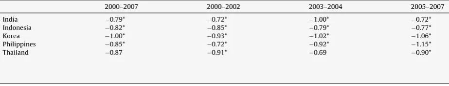
Managing price stability, especially for emerging economies with prohibitive vulnerability to sudden shifts in global investor sentiment, is imperative. The efforts to achieve this policy objective have been made more complex with unstable commodity prices and the global ﬁnancial meltdown, triggered initially by sub-prime mortgage defaults in the United States. A number of policy initiatives have been carried out. To rein in the unwanted consequences of volatile capital inﬂows on the local currencies in particular, and on the domestic economies in general, most of the major Asian economies were often

forced to resort to heavy sterilization (Table 1). However, facing the mounting cost and declining effectiveness of sterilization

measures, a number of these countries have gradually introduced more flexible regimes of exchange rate and carried out the necessary adjustments in their monetary, fiscal, investment and trade policies. For some emerging markets, the adoption of a more flexible exchange rate policy signified initial steps toward the full adoption of inflation targeting (IT) as the anchor of their monetary policies in particular and their macroeconomic policies in general.

Two of the most severely affected economies by the 1997 East Asian crisis, namely Indonesia and Thailand, have ofﬁcially adopted IT regimes. Although the process and the timing for the IT regime implementation varied between the two

A R T I C L E I N F O

Article history: Received 1 April 2008

Received in revised form 14 December 2009 Accepted 20 December 2009

JEL classiﬁcation: E52

E58 F31 F33

Keywords:

Inﬂationary expectation Output gap

Inﬂation targeting Pass-through Monetary policy rule

A B S T R A C T

The chief objective of our paper is to highlight basic features of the Information Technology (IT) policies adopted by Indonesia and Thailand, and to evaluate the commitment of the monetary authorities and the overall performances of the IT regime. The results demonstrate that the IT regime in these two economies has had some success, but not during the immediate aftermath of the Lehman Brothers’ collapse in the last quarter of 2008. Furthermore, the implementation IT policy in these economies has largely been ‘‘flexible’’ during the stable period, seeking the balance between narrowing the output gap, managing exchange rate volatility, and anchoring inflationary pressure. However during the turbulent period, there had been a heightened focus on anchoring inflationary expectations.

§

We are grateful to Bernard Ting, Shree Ravi and Seow Yun Yee for all research support. Comments from the anonymous referees of the journal on the early drafts are greatly acknowledged. Most of the early drafts were completed during the ﬁrst author’s stay at the International Monetary Fund-Singapore Training Institute, Singapore. The usual disclaimer applies.

* Corresponding author at: The SEACEN Centre, Lorong Universiti A, 59100 Kuala Lumpur, Malaysia. Fax: +60 3 7956 2755. E-mail addresses:[email protected],[email protected](R.Y. Siregar),[email protected](S. Goo).

Contents lists available atScienceDirect

Journal of Asian Economics

(2)

countries, the need to abandon the unsustainable rigid exchange rate policy, strengthen the operation of exchange rate policy, and improve effectiveness of monetary policy were among the common and principal motivations behind the adoption of the IT policy by these two major Southeast Asian countries.

There are two primary objectives of our paper. The ﬁrst one is to highlight the basic features of the IT policies adopted in Indonesia and Thailand, and to evaluate their overall performances, especially during the recent turbulent years. We will ﬁrst review a number of performance indicators such as price stability, growth rates and output volatility. Subsequently, our study will examine pass-through effects in both tradable and non-tradable prices, and effectiveness of the nominal exchange rate as a shock absorber.

The second objective is to examine the commitment of the monetary authorities of these two major Southeast Asian countries to implement the IT framework credibly. While this pertinent concern has been frequently debated in past studies, it has not been fully examined. The IT policy is credibly enforced if the monetary authority is committed to rein in

inﬂationary expectations as a primary or one of the key objectives of its monetary policy reaction function duringbothstable

and volatile economic environments (Bernanke & Mishkin, 2007; Schmidt-Hebbel & Tapia, 2002). Prior to 2007, a sustained

mild global inflation environment induced price stability in general and reduced potential trade-off and cost of having low inflation in the local economy. However, uncertainties about global economic conditions have heightened significantly, particularly since early 2007, posing challenges to policy efforts to manage price stability. Hence, it is pertinent to evaluate the commitment of these two countries to their implementation of the IT policy, and more importantly, to draw lessons on the effectiveness of the policy during the turbulent period of the past few years.

Recent studies have been conducted on the above list of issues. Yet, most of these early works focused their analyses mainly on the implementation of IT policy in the industrialized economies, and only a few have attempted to examine the

implementation of the IT regime in these two economies.1_{Our study hopes to ﬁll in the gap in the literature and ultimately}

aims to draw further policy lessons for the other emerging markets around the globe.

This paper proceeds as follows. The next section brieﬂy discusses policy backgrounds and basic economic performance indicators under the IT regime. Section three lays out the pass-through equation and the monetary policy rule framework to be tested in our study. The empirical section introduces the data sets and presents the ﬁndings of the autoregressive distributed lag (ARDL) for the pass-through effects. We employ the Markov-switching approach to examine the monetary reaction functions of the central banks. The test results allow us to compare and contrast the objectives of the monetary authorities of these two countries during the pre- and post-IT periods, and thus scrutinize their commitments to implement the IT policy. The last section concludes the paper.

2. Brief policy backgrounds and primary performance indicators

2.1. Policy backgrounds

2.1.1. Indonesia

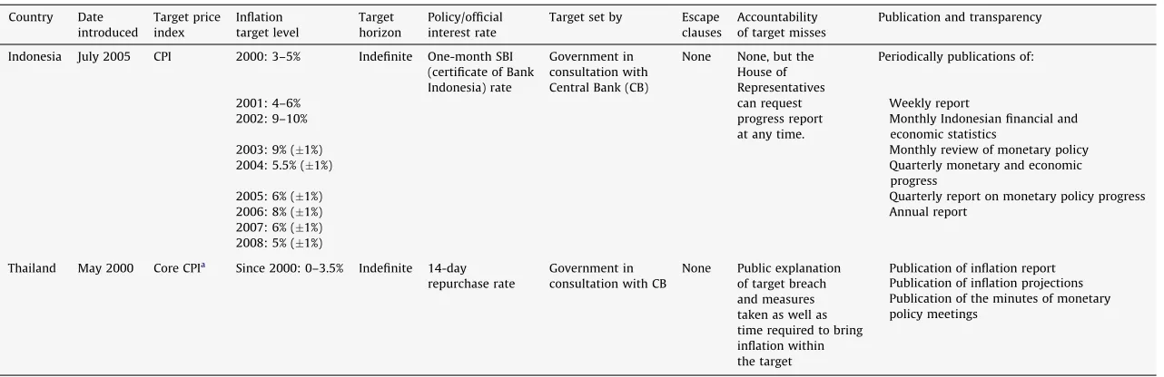
Bank Indonesia (BI), the monetary authority of Indonesia, officially launched its IT policy as its new monetary policy framework in July 2005. Under the IT framework, the inflation target represents the overriding monetary objective set by the Indonesian government in coordination with BI. The authorities have initially allowed the headline inflation to fluctuate

between the range of 91% in 2003, before gradually revising the headline inﬂation target downward to 51% for 2008 (Table 2).

Several reasons have been well documented as factors behind the move away from the past base money targeting framework to the current IT framework. To start, the effectiveness of the base money targeting policy of BI has signiﬁcantly

declined since the mid-1990s, especially during the period of the post-1997 East Asian ﬁnancial crisis.Boediono (1998)

underlined two reasons behind this. The ﬁrst has to do with the open market instrument. The markets for the central bank Table 1

Sterilization coefﬁcientsa,b .

2000–2007 2000–2002 2003–2004 2005–2007

India 0.79* 0.72* 1.00* 0.72*

Indonesia 0.82* 0.85* 0.79* 0.77*

Korea 1.00* 0.93* 1.02* 1.06*

Philippines 0.85* 0.72* 0.92* 1.15*

Thailand 0.87 0.91* 0.69 0.90*

Source: Asia Paciﬁc Regional Economic Outlook, IMF, October 2007. a

The sterilization coefficient is the coefficient from a regression on the contribution of net domestic assets to reserve money growth on the contribution of net foreign assets to reserve money growth. Net domestic assets in the regression are defined as reserve money minus net foreign assets.

b _{An asterisk denotes that the null hypothesis of full sterilization (a coefﬁcient equal to or smaller than}

1) cannot be rejected at the 95% conﬁdence level.

1

(3)

Table 2

Implementation and design of inﬂation targeting framework.

Country Date introduced

Target price index

Inﬂation target level

Target horizon

Policy/ofﬁcial interest rate

Target set by Escape clauses

Accountability of target misses

Publication and transparency

Indonesia July 2005 CPI 2000: 3–5% Indeﬁnite One-month SBI (certiﬁcate of Bank Indonesia) rate

Government in consultation with Central Bank (CB)

None None, but the House of Representatives can request progress report at any time.

Periodically publications of:

2001: 4–6% Weekly report

2002: 9–10% Monthly Indonesian ﬁnancial and

economic statistics

2003: 9% (1%) Monthly review of monetary policy

2004: 5.5% (1%) Quarterly monetary and economic

progress

2005: 6% (1%) Quarterly report on monetary policy progress

2006: 8% (1%) Annual report

2007: 6% (1%) 2008: 5% (1%)

Thailand May 2000 Core CPIa _{Since 2000: 0–3.5%} _Indeﬁnite _14-day repurchase rate

Government in consultation with CB

None Public explanation of target breach and measures taken as well as time required to bring inﬂation within the target

Publication of inﬂation report Publication of inﬂation projections Publication of the minutes of monetary policy meetings

Sources: Compiled by authors from the Bank Indonesia and the Bank of Thailand web-pages,Mishkin and Schmidt-Hebbel (2001),Ho and McCauley (2003). a

Thailand core CPI is deﬁned as CPI excluding raw food and energy prices.

Siregar,

S.

Goo

/Journal

of

Asian

Economics

21

(2010)

113–128

(4)

securities/bills (SBIs) and money market paper were relatively thin and segmented. The SBIs, in particular, were mostly held by the state banks in the mid- to late-1990s. Secondly, there were periods of pro-cyclicality of base money, where periods of upswings in the economy and rising aggregate demand were accompanied by both increased foreign borrowings and liquidation of SBIs, resulting in the excessive rise of the money supply.

In addition, the growing success of international experiences with IT countries in reining in inﬂation without increasing

output volatility had also inﬂuenced the decision to adopt the IT policy in Indonesia (Alamsyah et al., 2001). In particular, the

experiences of the pioneer group of IT economies, such as New Zealand, Australia and other industrial economies, demonstrate that with the rise in central bank credibility over time, IT policy reduces the variability of both inﬂation and

output (Cecchetti & Ehrmann, 1999).

To boost the effectiveness of monetary policy signals as well as to provide a greater market certainty, the BI rate was chosen as the interest rate instrument for Bank Indonesia. The BI rate is decided during the quarterly or monthly Board of Governors’ meeting, in response to the outlook for the achievement of the inﬂation target. Moreover, the BI rate is used as a reference in monetary control operations to ensure that the weighted average of one-month Certiﬁcate of Bank Indonesia (SBI) rate derived

in the Open Market Operations (OMOs) auctions remains at around the level of the BI rate.2_{Accordingly, the one-month SBI rate}

is expected to inﬂuence the interbank money market rates and the longer-term commercial interest rates.

2.1.2. Thailand

The Bank of Thailand (BOT) formally adopted its IT policy in May 2000 after exiting from the IMF ﬁnancial assistance programme. Similar to the case of Indonesia, the decision to shift from the previous monetary targeting regime to the current IT regime was largely driven by the recognition that the relationship between monetary indicators and output growth had became less stable, especially in the immediate aftermath of the 1997 ﬁnancial crisis and under the rapidly changing

ﬁnancial sector in Thailand (Charoenseang & Manakit, 2007; Kubo, 2008). In addition, the implementation of IT was deemed

necessary to restore BOT credibility as well as its independence (Jansen, 2001).

Under the IT framework, the quarterly average target of the core inﬂation (the headline inﬂation excluding raw food and

energy prices) has been set at a range of 0–3.5% from 2001 onwards (Table 2). The target bandwidth of 3.5% is expected to

mitigate temporary economic shocks and minimize the need for the BOT to carry out frequent monetary policy adjustments. The BOT sets the 14-day repurchase rate as its policy rate to inﬂuence the short-term money market rates. Furthermore, the monetary authority signals the shifts in its policy stance through the announced changes in the key policy rate via open

market operations (OMOs).3

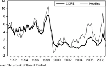
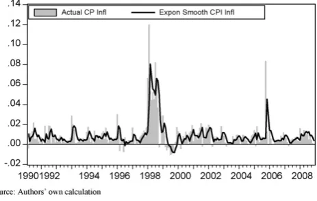
Looking at data from January 1991 through April 2000, the averages of the core inﬂation and headline inﬂation in Thailand

were relatively identical (McCauley, 2006). The maintenance of price stability in terms of core inﬂation, therefore, had been

expected to lead to stable headline inﬂation (Sriphayak, 2001). The recent episodes of the sub-prime ﬁnancial crisis and soaring

prices of key commodities have, however, challenged this early view on the stable relationship between core and headline

inﬂations in Thailand (Fig. 1). The average gap between the core and headline inﬂations in the country has not only widened,

especially since 2005, but it has become less stable as well.4_{We will come back to this issue at a latter stage of the paper.}

Fig. 1.Year on year core and headline inﬂations of Thailand.Source: The web-site of Bank of Thailand.

2

The monetary control operations take place through the use of the following instruments: (i) open market operations (OMOs), (ii) standing facilities; (iii) foreign exchange market intervention, (iv) establishment of the minimum statutory reserve requirement, and (v) moral suasion. The most important monetary control instrument is the OMOs. BI began issuing its own debt in the form of SBI to manage the money supply since 1984. Currently, the one-month SBI is auctioned weekly while the three-one-month SBI is auctioned one-monthly.

3

In conducting the open market operation, the BOT undertakes transactions in the ﬁnancial markets to affect the aggregate level of reserve balances available in the banking system and thus affecting the short-term interest rates.

4

(5)

2.2. Preliminary performance indicators

A number of basic performance indicators have often been applied to evaluate the outcome of the inﬂation targeting

policy. Most have considered the potential trade-offs between economic growth and inﬂation. Cecchetti and Ehrmann

(1999), for instance, argue that one should expect to see a heightened volatility of output in the IT countries as the monetary

authorities manipulated the output gap to reverse shocks to inﬂation. Similarly, Mishkin and Schdmit-Hebbel (2007)

examine both the mean and the standard deviation of the inﬂation rate and the GDP growth rate during the pre-and post-IT periods to analyze growth and volatility, as well as the potential trade-offs between them. For the IT policy to be considered successful, the following outcomes should at least be achieved:

Lower inﬂation and output volatility are achieved during the post-IT when compared to the pre-IT rates.

The sacriﬁce ratio (i.e. the output cost of maintaining inﬂation rate within the targeted range) declines over time.

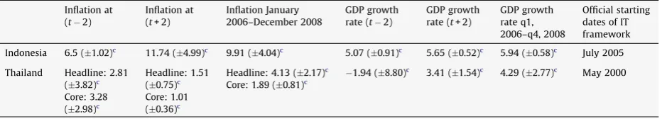
Table 3reports the mean (the growth) and standard deviation (the volatility) of the annualized monthly consumer price index (CPI)-based inﬂation and the annualized quarterly GDP growth rate for both economies during the period of two years

before (t2) and after (t+ 2) of the full adoption of the IT policy. FollowingIMF (2005), two features/conditions must be met

for a full-ﬂedged IT regime:

(a) The central bank is mandated and committed to a unique numerical target in the form of a level or a range of annual inﬂation, and

(b) The inﬂation forecast over some horizon is the de facto intermediate target of monetary policy.

The ofﬁcial starting dates of the IT framework in Indonesia and Thailand reported inTable 2meet these two conditions.

We ﬁnd several consistent and contrasting ﬁndings:

1 In general, we found inﬂation rates in Thailand, but not in Indonesia, to be relatively lower and less volatile during the two immediate years following the adoption of the IT policy rather than during the pre-IT period. Since the target is the core

inflation,Table 3reports both core and headline inflation for the case of Thailand. The high inflation rate at (t+ 2) in

Indonesia was driven by signiﬁcant cuts on subsidies for fuel and related products in the second quarter of 2005. 2 Most encouragingly, there seems to be no trade-off between inﬂation and economic growth. The average GDP growth rates

of Indonesia and Thailand during (t+ 2) were signiﬁcantly higher and less volatile (smaller standard deviations) than the

rates during the pre-IT period.

3 The headline inflation rates in these two economies had risen significantly in recent years. For Indonesia, the mean of the annualized headline inflation had been well above the target rate, especially starting the second half of 2008. The rise in the key commodity prices in the world market contributed significantly to the sudden rise in the domestic inflations of the two

Southeast Asian economies.5_{From January 2007 to January 2008, the average headline inﬂation rate in Indonesia was still}

hovering well within the target of Bank Indonesia, at around 6%. The inﬂation rate had, however, almost doubled during the second half of 2008.

Table 3

Pre- and post-IT headline inﬂation and GDP growth rates at (t2) to

(t+ 2)a

(mean and standard deviation)b .

Inﬂation at (t2)

Inﬂation at (t+ 2)

Inﬂation January 2006–December 2008

GDP growth rate (t2)

GDP growth rate (t+ 2)

GDP growth rate q1, 2006–q4, 2008

Ofﬁcial starting dates of IT framework

Indonesia 6.5 (1.02)c _{11.74 (}

4.99)c _{9.91 (}

4.04)c _{5.07 (}

0.91)c _{5.65 (}

0.52)c _{5.94 (}

0.58)c _{July 2005}

Thailand Headline: 2.81 (3.82)c Core: 3.28 (2.98)c

Headline: 1.51 (0.75)c Core: 1.01 (0.36)c

Headline: 4.13 (2.17)c Core: 1.89 (0.81)c

1.94 (8.80)c

3.41 (1.54)c

4.29 (2.77)c

May 2000

Source: Authors’ own calculation and the web-sites of Bank Indonesia and Bank of Thailand. a

(t2) denotes two years prior to the adoption of inﬂation targeting framework and (t+ 2) implies two years after the adoption of IT framework. b

Mean for inﬂation is calculated as the monthly average of year on year inﬂationðDp¼ ½ðCPItCPIt12Þ=CPIt12 100Þ. The mean for GDP growth rate is the average of the annualized quarterly GDP growth rateðDGDP¼ ½ðGDPtGDPt4Þ=GDPt4 100Þ.Note: GDP is in local currency at constant market price.

c

The numbers inside () are the standard deviation.

5

(6)

4 Despite the rise in the headline inflation, the core inflation rate continued to remain well below the inflation target of Bank of Thailand in recent years. There has, indeed, been a marked increase in the core inflation and a significant widening gap between the core and the headline inflation, capturing the steep rise in the non-core inflation driven by the escalated and

volatile commodity prices between 2006 and 2008 (Fig. 1).

5 Although the overall growth rates remained strong for the full year of 2008, we have seen adverse impacts of the global financial crisis (especially since September 2008 with the closure of the Lehman Brothers) and the volatile prices of key commodities. The final quarter of 2008 has witnessed the annualized GDP growth rate of Thailand to contract by about 4%. The recent experiences with high inflation and low growth reconfirm the concern over the effectiveness and superiority of inflation target regime over other monetary regimes during the episodes of economic turbulences.

3. Working model

3.1. Inﬂation inertia and pass-through effects

To further examine the performance of the IT policy, our next task is to examine the pass-through effects in these two economies. Has the IT regime reduced the pass-through effects and inﬂation inertia, and therefore contributed to the

reported fall in the domestic inﬂation rates of these two economies?Taylor (2000)argues that the extent of a

pass-through decline is highly inﬂuenced by the strong commitment of the monetary authority towards price stability.

Supporting Taylor’s claim,Gagnon and Ihrig (2004)tested a sample of advanced nations and found that the decline in

the pass-through related to the changes in monetary policy procedures, and in particular, to the adoption of inﬂation targeting.

Edwards (2006), however, demonstrates that ‘‘pass-through problem’’ does not only relate to the issue of inflation, but also to the overall effectiveness of the nominal exchange rate as a shock absorber. The study, therefore, argues that it is important to make a distinction between the pass-through of exchange rate changes into the domestic price of non-tradables and the domestic price of tradables. From a policy perspective, a desirable situation is to attain a more efficient shock absorbing exchange rate where the pass-through coefficients for tradable and non-tradable are low and different, with the pass-through for tradable goods being higher than that for non-tradable goods.

To address the set of questions introduced earlier, our study employs the following empirical model based onEdwards

(2006)6_:

D

logPt¼

b

0þ X

n

i¼1

b

1i

D

logEtiþ

X

n

i¼1

b

2ilog

D

Ptiþ

X

n

i¼1

b

3ilog

D

Ptiþ

X

n

i¼1

b

4ið

D

logEtiDITÞ þ

X

b

5ið

D

logPtiDITÞ þ

e

_t

(1) where

Ptis a domestic price index – either of tradable or tradable. As proxies, the rate of change of the CPI is for the

non-tradable inﬂation, and the rate of change for the producer price index (PPI) is for the non-tradable inﬂation.

Etis the nominal effective exchange rate (an increase implies a nominal depreciation of the local currency).

P

tis a world price index. The change of this index captures the rate of world inﬂation. The US consumer price index will be

adopted here as a proxy.

DITis a dummy variable for the Inﬂation Targeting regime. It is equal to zero before the adoption of the inﬂation target in

the country, and equals to one otherwise.

Several fundamental assessments can be derived from the regression outcomes on Eq.(1):

The ﬁrst is the pre-IT short-run pass-through, captured byP

b

1. We would expect

P

b

1to be equal or greater than zero, i.e. a

depreciation of the nominal effective exchange rate (

D

logE>0) would lead to a rise in the inﬂation (

D

logP>0) and vice

versa.

The second is the post-IT short-run pass-through P

b

1þ P

b

4

ð Þ. If P

b

4<0

ð Þ, the pass-through effect for the post-IT

period is lower than that of the pre-IT. Hence, we ﬁnd evidence to supportTaylor (2000), that a more inﬂationary-focused

policy such as IT should reduce pass-through.

The third one is the pre-IT long-run pass-through, estimated as P

b

1=ð1 P

b

3Þ

ð Þ:Similar to the short-run pre-IT

pass-through, we would expect the long-run pre-IT pass-through to be positive.

The next one is the long-run pass-through estimates for the post-IT period, P

b

1þ P

b

4

ð Þ=1 P

b

3þ P

b

5

ð Þ

ð Þ.

P

b

1=ð1P

b

3Þ

ð Þ> P

b

1þP

b

4

ð Þ=1 P

b

3þP

b

5

ð Þ

ð Þimplies that the adoption of the IT policy has reduced the

long-run pass-through effects.

P

b

5>0 suggests that inﬂation inertia has risen in the local economy. The rise (fall) in inﬂation inertia may contribute as

well to the rise (fall) in the long-run pass-through during the post-IT as compared to the pre-IT period.

(7)

Lastly, we will evaluate whether the ratio of the pass-through coefﬁcients for the non-tradable price over those of the tradable prices has declined (increased), suggesting that the nominal exchange rate is becoming a more (less) efﬁcient shock absorber.

3.1.1. Robustness testing: the degree of economic openness

Early works such asCampa and Goldberg (2002),Gagnon and Ihrig (2004),Frankel, Parsley, and Wei (2005)andBIS (2005)

among others, have recorded a broad-based decline in the exchange rate pass-through (ERPT) during the past two decades. These studies offer a number of plausible explanations for the decline in the ERPT, but most of them consistently underline the signiﬁcant contribution of import penetration, international mobility of capital, and overall degree of economic openness.

Given the possibility that the degree of economic openness may have contributed to a possible fall in the size of the exchange rate pass-through in our two economies, it is therefore warranted to ensure the robustness of our test results that

the openness variable is added as a control variable in Eq.(1)7_:

D

logPt¼

b

0þ Xn

i¼1

b

1i

D

logEtiþ

Xn

i¼1

b

2ilog

D

Ptiþ

Xn

i¼1

b

3ilog

D

Ptiþ

Xn

i¼1

b

4ið

D

logEtiDITÞ þ

Xn

i¼1

b

5i

D

logPtiDIT

þX

n

i¼1

b

6ið

D

O pennessÞ þ

e

t (2)

The (Openness) control variable for Indonesia and Thailand would capture the impact of both trade and ﬁnancial sector

reforms on the degree of economic openness of the countries. The monthly (Openness) variable is calculated as the product of

log-normalized values of export (lnExportt), import (lnImportt) and market capitalization of the stock exchanges

(lnMarketCapt), hence (Opennesst= lnExporttlnImporttlnMarketCapt).8Accordingly, the rate of change in the degree of

the economic openness is calculated as (

D

Opennesst=OpennesstOpennesst1). As the rise in the degree of the economic

openness should reduce the inﬂationary pressure in the local economy, the sign of the coefﬁcient estimate (

b

6) is expected to

be negative.

3.2. Monetary policy reaction function under inﬂation targeting policy

Can the decline in the inﬂation rate and the pass-through effect during the IT period be attributed to the full commitment of the monetary authority to the pursuit of its IT policy? One way to address this question is by examining the monetary

policy rule of the central bank during the pre- and the post-IT period.Taylor in his 1993seminal paper, proposes a very

speciﬁc and simple monetary policy rule, where the central bank adjusts its key interest rate in a smooth manner responding to the changes in the expected inﬂation and output gap. Furthermore, his study and many others, have argued that the

domestic monetary policy does not systematically respond to external shocks.9_{Therefore, the exchange rate variable should}

not be explicitly included in the reaction function of the monetary authority. The arguments are two folds. First, the exchange rate should already play an indirect role through the inﬂation and output variable. Second, adding the exchange

rate into the policy rule will only place considerably more volatility to monetary policy (Taylor, 2001).Mishkin and

Schmidt-Hebbel (2001)shared this view as well. Likewise,Clarida (2001)contends that even though central banks do not target the exchange rate explicitly, the central banks’ objective to stabilize inﬂation will lead to the increase in short-term interest rate when the domestic currency is weakening and vice versa.

Others, however, challenge the exclusion of the exchange rate in the optimal monetary policy rule.Svensson (2000)for

instance, argues the need to allow for the indirect and direct exchange rate transmission channel in the optimal monetary policy reaction function. In his 1993 seminal paper, Taylor had initially allowed for a signiﬁcant role of the exchange rate factor in the policy reaction function of the Federal Reserve Board (FRB). Due to its adverse implication on the overall performance of the macroeconomic performance when the FRB reacted too strongly to the exchange rate, the study eventually omitted the exchange rate in the 1993 rule for the FRB. However, Taylor acknowledges that ‘it is not clear that the

same conclusion would hold for other countries’ (Taylor, 2001). The importance of exchange rate factor has also been

underscored in a recent study ofAizenman, Hutchison, and Noy (2008).

For our study, there are a number of compelling reasons to explicitly account for the role of the exchange rate variable in the monetary policy reaction function. To start with, external shocks are transmitted largely through exchange rate

7

Investment and Trade reforms in Indonesia and Thailand had taken place rapidly in the mid-1980s and were followed by aggressive liberalization of the ﬁnancial sector, particularly in the banking and capital market. Both economies shifted away from import-substitution policy to export promotion in 1980s and committed themselves to both multilateral trade arrangements (such the World Trade Organization (WTO) and the Asia Paciﬁc Economic Cooperation (APEC) in 1990s), and bilateral trade arrangements with their key trading partners, such as the USA and Japan in 2000s (Sen & Rajan, 2005; Kastner & Kim, 2008). As an annual percentage of GDP, the average total export and import surged from the levels of around 36% and 53% in 1985–1990 in Indonesia and Thailand, respectively, to as high as around 45% and 118% in 2002–2007. Much more impressive trends have been demonstrated by the market capitalizations of the stock exchanges in these two Southeast Asian nations. The capitalizations of the Jakarta Stock Exchange and the Bangkok Stock Exchange which were averaging around 0.10% and 3% per annum of GDP in 1980–1985, surged to 30% and 67%, respectively, in 2002–2007.

8

Given that there are no monthly ofﬁcial GDP data for both economies, we are not able to calculate the composition of the (Openness) control variable as monthly percentages of GDP.

(8)

movements in small open economies such as Indonesia and Thailand. More importantly, the monetary authorities of these economies had officially and unofficially adopted rigid exchange rate policy regimes in the past. Hence, by including the exchange rate variable, we can examine whether the monetary authorities continued to place a significant weight on the exchange rate variable during the IT period.

To test the monetary policy reaction function, we adopt an approach introduced byClarida, Gali, and Gertler (1998),

henceforth refer to as the CGG approach10_:

rt¼rtþ

X

n

i

di

Etiptþ1iþ

X

n

i

f

iðEtiytþ1iyÞ þ

X

n

i

z

tðqtiÞ þ

e

t (3)

where:ris the short-term policy interest rate target;r

t is the desired nominal interest rate;Et

p

t+1andEtyt+1are expected

inﬂation and output for period (t+ 1), respectively, conditioned on information set available at time (t); (y*) is the potential

output; (qti) denotes the lagged real exchange rate ﬂuctuation, captured by the periodical percentage change of the real

effective exchange rate.11_{A positive (}_q_{) implies a weakening of the local currency.}

d

_,

f

_and

z

_{are the parameters signaling the}

central bank’s response to deviations of expected inﬂation from inﬂation targets, expected output gap and past exchange rate volatilities, respectively.

Early studies have demonstrated that under forward looking expectation, interest rate smoothing behavior, such that

rt¼ ð1

r

Þrtþ

r

ðLÞrtiþ

e

_t, should have a stabilizing effect on the monetary policy reaction function (Clarida et al., 1998;

Rudebusch & Svensson, 1999). Incorporating interest rate smoothing into Eq.(3), the following monetary policy reaction function can be speciﬁed:

rt¼

v

þ

X

n

i

r

irt1iþ

X

n

i

di

Etiptþ1iþ

X

n

i

f

iðEtiytþ1iyÞ þ

X

n

i

z

tiðqt1iÞ þ

e

t (4)

wherertis the current interest rate,

r

2[0,1] captures the interest rate smoothing behaviour.12

Eq.(4)basically indicates that the key central bank interest rate will be determined by the past levels of interest rate and

exchange rate volatility, and the past and present levels of expected inﬂation rate and expected output gap. Based on the

signiﬁcance and the size of the estimate coefﬁcients of

r

,

d

,

f

and

z

, we can analyze the relative weights of these key

economic indicators on the monetary policy rule of the country. Theoretically, we would expect

d

,

f

and

z

to be all positive.

The rise in the inﬂation expectation should lead to the tightening of monetary policy. Similarly, rising expected output gap

(Etiyt+1y*) should result in stronger inﬂationary pressure, and therefore requires a tighter monetary policy stance. Lastly,

a positive rise in (q) should trigger stronger imported inﬂation and warrants an upward adjustment in the key interest rate.

To ensure consistent analyses, we consider the implementation of the IT policy to be credible if and only if the expected inflation variable is significant during both regimes, i.e., the forward looking policy to rein in inflation should always be fully enforced under both stable and volatile economic conditions. In an extreme case where an IT country places a significant

weight only on the inﬂation variable, this country then, according to literature, is following the ITrule.On the other hand, the

implementation of the IT policy would be considered a ﬂexible one – following the ITframework, when there is a

discretionary space for the monetary authority to place more important weights on other factors, such as output stability or

exchange rate volatilities, than on price stability (Bernanke & Mishkin, 2007).13_{Naturally, if none of the above conditions is}

met, then IT policy has not been enforced. Accordingly, one can argue that other factors, such as a more stable macroeconomic environment, are largely responsible for the low inﬂation and the more moderate pass-through effects.

4. Empirics

4.1. Data and date selection

Our monthly data series run from January 1990 to December 2008. Most of the raw data for prices, key interest rates and exchange rates are sourced from the ofﬁcial web-sites of the central banks of the individual countries and the International Financial Statistics (IFS) of the International Monetary Fund. However, due to the lack of ofﬁcial data, the nominal and real

effective exchange rates of Indonesia are sourced from the database of JP-Morgan. As discussed earlier, we followIMF (2005)

on the selection of the starting dates for the ofﬁcial implementation of the IT policy.

All raw variables are in the log-form. The inﬂation rate is calculated as the monthly percentage change in the price levels (consumer price index (CPI) and producer price index (PPI)). The monthly industrial production index (IP) for each country is adopted to proxy the domestic output, and the growth rate is calculated as the monthly percentage change of the IP. For the key policy rate, we employ the three-month SBI rate for Indonesia and the 14-day repurchase rate for Thailand.

10_{As brieﬂy mentioned, the CGG approach is often referred to as an augmented version of the Taylor rule with forward looking expectation on inﬂation,} output and exchange rate gaps (refer toTaylor, 2001; Chadha, Lucio, & Valente, 2004).

11

Managing volatility of the local currency has indeed been part of the critical feature of IT policy in both Indonesia and Thailand (Alamsyah et al., 2001; Charoenseang & Manakit, 2007).

12

Refer toClarida et al. (1998)for the full derivation from Eqs.(3) to (4).

(9)

4.2. Autoregressive distributed lag approach for pass-through and inﬂation inertia

4.2.1. Exponential smoothing inﬂation ofCogley (2002)

Most studies examining the pass-through effects for developing countries often rely on the most common measure of inflation such as the CPI-based or PPI-based rates of inflation. However, it is well known that there is a substantial presence of transient noises in the CPI series of developing economies, due for instance to the relatively larger shares of household expenditures on food and energy products. The volatility of the world prices of food and energy commodities, especially since mid-2005, has indeed contributed to the much more volatile CPI series in Indonesia and Thailand in recent years. Therefore, to enhance the quality of our pass-through estimates, in addition to the CPI and the PPI-based inflation series, we also calculate the exponentially smoothed version of the CPI and PPI-based inflation series as

proposed by Cogley (2002).

Extending the early works ofBryan and Cecchetti (1995)andCecchetti (1997),Cogley (2002)proposes a simple adaptive

method for ﬁltering inﬂation data to remove transient noise. The study demonstrates that by considering the source of

persistentmovements in inﬂation, it can further reduce the still relatively high-frequency variation of the transient noise in

the inﬂation series derived from the earlier approach ofBryan and Cecchetti (1995).14

Cogley (2002)develops a core measure of inflation that down-weights distant movements in the price index. The study proposes the following core inflation measure, involving the exponential smoothing of current and past aggregate inflation series:

˜

pt

¼g0X

j¼0

ð1g0Þj

p

tj; 0<g0<1 (5)

where

p

denotes the relevant aggregate CPI or PPI-based inﬂation rates. Eq.(5)deﬁnes the core measure as a one-sided

geometric distributed lag of current and past inﬂation.Cogley (2002)sets the gain parameter ofg0= 0.125. For our study,

however, we do not predetermine the size ofg0. Instead we estimate the smoothing parameter (g0) that will minimize the

sum of squares of one-step forecast errors.

Figs. 2 and 3contrast and compare the monthly inﬂation rates based on the actual CPI against that derived by the

exponentially smoothing approach ofCogley (2002). Clearly, a fair amount of transient noises in the CPI-based inﬂation rates

of Indonesia and Thailand has successfully been taken out by the smoothing process. For the sake of brevity, we do not report

the exponential smoothed inflation figures based on the PPI series.15_{Given these results, the inflation series employed in our}

pass-through testing will be that of the exponentially smoothed series of the tradable and non-tradable inﬂation series.

4.2.2. Pass-through effects

Early studies have acknowledged that (

D

logE) may not be exogenous in Eq.(2)and may very well be correlated with the

error term. However, ﬁnding an appropriate instrumental variable for (

D

logE) is difﬁcult.16_{One way to circumvent the}

problem is to employ the classical ARDL testing with the general to speciﬁc approach (Hendry, 1976). This is a common

approach adopted by early studies such asCampa and Goldberg (2002)andGagnon and Ihrig (2004). To avoid potential

Fig. 2.Monthly CPI-based inﬂation in Indonesia (lnPtlnPt1).Source: Authors’ own calculation.

14_{Since the CPI index for each component of the aggregate CPI index is not officially available for Indonesia (full data only available starting 2000) and} Thailand (only 7 components are available), we are not able to calculate the weighted median measure of the aggregate inflation series proposed byBryan and Cecchetti (1995)for both of these economies. Moreover, given that the adaptive measure ofCogley (2002)has demonstrated to successfully generate less volatile inflation series than the approach ofBryan and Cecchetti (1995), we will only employ the former methodology.

15

These ﬁgures can be made available upon request.

(10)

endogeneity, the ARDL testing includes variables at period (t1i) only, withi= 0,. . .,n.

17_{In addition, a crisis dummy is}

included in the testing to capture potential structural breaks due to the ﬁnancial and exchange rate crisis which started in the middle of 1997. Furthermore, a battery of test statistics will be reported to ensure that our coefﬁcient estimates are valid and robust.

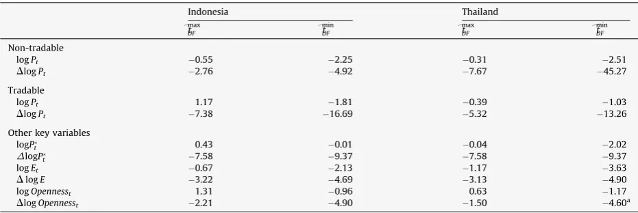
Prior to conducting the ARDL testing, we test the unit-root properties for each of the variables in Eq.(2). To anticipate

possible presences of structural breaks, we employBanerjee, Lumsdaine, & Stock (1992)– henceforth BLS, in addition to

standard unit-root tests, i.e. the ADF-test, the Phillip Perron test and the KPSS test.18_{Depending on the unit-root properties of}

the series, we then test for the possible cointegrating relationship among the variables in Eq.(2). If cointegrating relationship

is found, then the error-correction component series (ECMt1) will be included in the ARDL testing.

Based on our set of unit-root tests, all relevant series are all found to be non-stationary and integrated of order 1 at their

level—I(1) series (Table 4).19Furthermore, the (Opennesst) variable is also tested to be non-stationary at the level, hence

having a consistent unit-root property with the rest of the variables in Eq.(2). Furthermore, with the exception of the case of

the tradable price of Indonesia, we ﬁnd weak evidences of cointegrating relationship in Eq.(2). Accordingly, the

error-correction component is included in the ARDL regression. The pass-through test results are reported inTables 5 and 6.20_The

Table 4

BLS-rolling unit-root test results.

Indonesia Thailand

t

_max

DF t

_min

DF t

_max

DF t

_min DF

Non-tradable

logPt 0.55 2.25 0.31 2.51

DlogPt 2.76 4.92 7.67 45.27

Tradable

logPt 1.17 1.81 0.39 1.03

DlogPt 7.38 16.69 5.32 13.26

Other key variables logP

t 0.43 0.01 0.04 2.02

DlogP

t 7.58 9.37 7.58 9.37

logEt 0.67 2.13 1.17 3.63

DlogE 3.22 4.69 3.13 4.90

logOpennesst 1.31 0.96 0.63 1.17

DlogOpennesst 2.21 4.90 1.50 4.60a

Source: Authors’ own calculation.

Notes: Critical value for the maximal DF statistics at 5% level for total observation set of around 250 (or less) is (1.48) and critical value for the minimal DF statistics at 5% for the same set of observation is (4.85). Our total observation set is around 220.

a__tmin

DF is lower than the critical value for the minimal DF statistics at 10%.

Fig. 3.Monthly CPI-based inﬂation in Thailand (lnPtlnPt1).Source: Authors’ own calculation.

17_{Due to the degree of freedom, we start with}_{i= 5 (up to six month lag). In all cases, we do not ﬁnd higher lagged variables to be signiﬁcant.} 18_{The BLS provides a more in-depth investigation of the possibility that the aggregate economic time series can be characterized as being stationary} around ‘a single or multiple structural breaks’. It extends the Dickey–Fullert-test by the construction of the time series of rolling computed estimators and theirt-statistics. Following the BLS procedure, we compute the smallest (minimal) and the largest Dickey–Fullert-statistics.

19

For the sake of brevity, the results of the standard unit-root tests will not be posted, but they can be made available upon request. 20

(11)

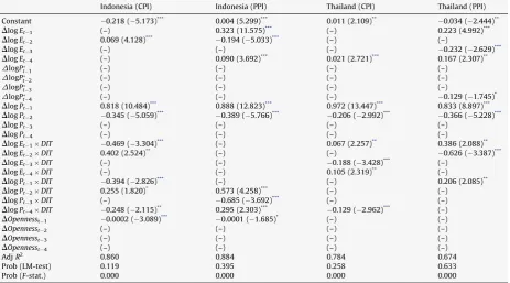
R2_{values suggest that the explanatory variables can clarify on average, around 80% of the monthly price changes of tradable}

and non-tradable goods. TheF-statistics indicate that one or more of the independent variables are non-zero. In addition, the

Breusch–Godfrey serial correlation LM-test statistics conﬁrm that autocorrelations in the residuals are not a problem in any of the regressions.

Supporting the claims ofTaylor (2000)andGagnon and Ihrig (2004), our test results suggest that the short- and long-run

pass-through effects for the non-tradable prices have all declined in the post-IT periods in these two economies (Table 6). The

rates of changes for short-run pass-through P

b

1þ P

b

4

ð Þ P

b

1

ð Þ and long-run pass-through effects

P

b

1þ P

b

4

ð Þ=1 P

b

3þ P

b

5

ð Þ

ð Þ P

b

1=1 P

b

3

ð Þ

ð Þare in the ranges of (0.067 to0.129) for Indonesia and

(0.016 to0.048) for Thailand. Similar evidences are reported as well from the tradable price of Thailand, but not for the

case of Indonesia.

The effectiveness of the IT policy in mitigating inﬂation inertia has also been demonstrated in the two countries for the case of non-tradable price. Yet, the policy has had limited success in anchoring inﬂation inertia in domestic tradable prices of

these two Southeast Asian nations. Inﬂation inertia P

b

5

ð Þfor the tradable price has in fact increased by about (0.18) and

(0.21) for Indonesia and Thailand, respectively, during the post-IT period. Table 5

Pass-through effects.

Indonesia (CPI) Indonesia (PPI) Thailand (CPI) Thailand (PPI)

Constant 0.218 (5.173)***

0.004 (5.299)***

0.011 (2.109)**

0.034 (2.444)**

DlogEt1 (–) 0.323 (11.575)*** (–) 0.223 (4.992)***

DlogEt2 0.069 (4.128)*** 0.194 (5.033)*** (–) (–)

DlogEt3 (–) (–) (–) 0.232 (2.629)***

DlogEt4 (–) 0.090 (3.692)*** 0.021 (2.721)*** 0.167 (2.307)**

DlogP

t1 (–) (–) (–) (–)

DlogP

t2 (–) (–) (–) (–)

DlogP

t3 (–) (–) (–) (–)

DlogP

t4 (–) (–) (–) 0.129 (1.745)

* DlogPt1 0.818 (10.484)*** 0.888 (12.823)*** 0.972 (13.447)*** 0.833 (8.897)*** DlogPt2 0.345 (5.059)*** 0.389 (5.766)*** 0.206 (2.992)*** 0.366 (5.228)***

DlogPt3 (–) (–) (–) (–)

DlogPt4 (–) (–) (–) (–)

DlogEt1DIT 0.469 (3.304)*** (–) 0.067 (2.257)** 0.386 (2.088)**

DlogEt2DIT 0.402 (2.524)** (–) (–) 0.626 (3.387)***

D_log_E_t₃_DIT _(–) _(–) _{0.188 (}_3.428)***

(–)

DlogEt4DIT (–) (–) 0.105 (2.319)** (–)

DlogPt1DIT 0.394 (2.826)*** (–) (–) 0.206 (2.085)**

DlogPt2DIT 0.255 (1.820)* 0.573 (4.258)*** (–) (–)

DlogPt3DIT (–) 0.685 (3.692)*** (–) (–)

DlogPt4DIT 0.248 (2.115)** 0.295 (2.303)*** 0.129 (2.962)*** (–) DOpennesst1 0.0002 (3.089)*** 0.0001 (1.685)* (–) (–)

D_Openness_t₂ _(–) _(–) _(–) _(–)

D_Openness_t₃ (–) (–) (–) (–)

DOpennesst4 (–) (–) (–) (–)

AdjR2

0.860 0.884 0.784 0.674

Prob (LM-test) 0.119 0.395 0.258 0.633

Prob (F-stat.) 0.000 0.000 0.000 0.000

Note: (–) implies not signiﬁcant, hence excluded from the ﬁnal test; ()t-statistics. *

10% significant. ** _{5% significant.} *** _{1% significant.}

Table 6

Summary of impact of IT on the pass-through *******effectsa .

IT impact on short-run pass-through IT impact on long-run pass-through Inﬂation inertia

P b1þPb4

ð Þ P

b1

P b1þP

b4

1P_b 3þP_b

5 ð Þ P b1

1P_b 3

: P

b5 1. Non-tradable

Indonesia 0.067 0.129 0.387

Thailand 0.016 0.048 0.129

2. Tradable

Indonesia 0.000 0.251 0.183

Thailand 0.240 0.547 0.206

(12)

There is also no conclusive evidence that the nominal exchange rate has become a more efﬁcient shock absorber. As highlighted, the nominal exchange rate is considered to be a more efﬁcient absorber, if the rates of decline in both short- and long-run pass-through effects of the non-tradable prices are larger than those reported for tradable prices. This is not the case for Thailand. Similarly, the evidence is at most a weak one for the case of Indonesia, as the pass-through effects for the tradable price in Indonesia continued to rise during the post-IT period.

The overall ARDL test results seem to suggest that the inflation targeting policy in Thailand has, in general, shown more favorable outcomes. It is interesting to note, however, that the less encouraging results for the IT policy performance in Indonesia, are largely consistent with the prevailing stylized facts. To begin, the IT policy has only officially been launched in July 2005, about five years later than when it was first initiated in Thailand. Furthermore, the IT policy was first implemented during the time when the government of Indonesia initiated its gradual reductions of various energy subsidies. The measure has successfully alleviated pressures on the current expenditure of the central government budget, but at the cost of rising transportation and production costs, and eventually increasing the prices of key commodities, including food products, especially during the episodes of unprecedented surges in the prices of various energy commodities, between late 2007 to middle of 2008. The rise in the non-tradable price has in turn, further fueled inflationary pressure on the overall headline

inﬂation in the country (Table 3).

4.2.3. Robustness testing: the role of openness

As discussed, to ensure the robustness of our pass-through test results and that the pass-through effects have not been

over-estimated, we include the Openness variable in Eq.(2). We ﬁnd that the coefﬁcient estimate of the Openness variable

(

D

Opennesst) to be signiﬁcant only for the case of Indonesia (Table 5). The negative coefﬁcient signs seem to support the early

ﬁndings ofCampa and Goldberg (2002),Gagnon and Ihrig (2004),Frankel et al. (2005)andBIS (2005)that the rise in the

overall degree of openness should dampen inﬂationary pressure domestically.

It is important to emphasize here, however, that those previous assessments on the degrees of the pass-through effects and inﬂation inertia, and the roles of IT policy in explaining their changes from the pre- to post-IT periods have been based on the assumption that the monetary authorities of these two countries have, indeed, been committed in implementing the IT policy. This is clearly a brave assumption that needs to be examined, and the objective of the next step of our study is to do so.

4.3. Markov-switching approach for monetary policy rule

To compare and contrast the experiences and the shifts in the policy rules under the pre- and post-IT periods, past studies, in general, separated the sample observations into two sets, that is, the and the post-IT periods based on the pre-determined starting dates of the IT policy. This approach, however, would lead to a potential problem with the degree of freedom. For the case of Indonesia in particular, we will not be able to carry out any testing for the post-crisis period as Indonesia only ofﬁcially adopted the IT policy in July 2005. By breaking the samples into the pre- and post-IT groups, we would not have enough degrees of freedom to carry out any testing for the post-IT period. To avoid the above shortcomings,

we employ the Markov-switching (MS) regression procedure for Eq.(4). The MS-VAR does not require us to break the

observations into two sample sets as it is designed to pick out changes in the generating mechanism of a series. In our case, the changes in the central bank’s operating rule will almost certainly affect the stochastic process of the short-term interest

rate in Eq.(4).

Furthermore, the dynamics of the interest rate may change from a period of stability to that of volatility.21_{Understanding}

the change is critical in our efforts to assess the commitment of the central banks in implementing IT policy. As discussed earlier, the monetary authority is committed to IT if and only if they continue to place a signiﬁcant weight on inﬂation during both stable and turbulent periods.

The Markov-switching VAR framework is essentially extendingHamilton’s (1989)Markov-switching regime framework

to the Vector Autoregressive (VAR) systems (seeKrolzig, 1997; Sims, 1999; Valente, 2003). Our study considers three types of

MS-VAR models that allow for either regime shifts in the intercept term, variance-covariance matrix or autoregressive terms.

Firstly, we will consider aM-regimepth order Markov-switching VAR that allows for regime shifts in variance-covariance

matrix. The Markov-switching-heteroscedastic-VAR or MSH(M)-VAR(p), may be written as follows:

yt¼

v

þ

X

p

i¼1

Aiytiþ

e

t (6)

whereyt is aK-dimensional observed time-series vector,yt= [y1t,y2t,. . .,yKt]

0 _{and for this paper matrix}_y

tcontains all

variables used in our monetary policy reaction functions (see Eq.(4)).vis aK-dimensional column vector of intercept terms,

v

¼ ½

v

₁_;

v

₂_{; :::;}

v

_K0; theAis areKKmatrices of autoregressive parameters;

e

_t= [

e

₁t,

e

₂t,_{. . .},

e

Kt]0is aK-dimensional vector

of Gaussian white noise process with a regime-dependent variance-covariance matrix

S

,

e

NID(0,

S

(s_t)). The

21

(13)

regime-generating process is assumed to be a hidden Markov chain with a ﬁnite number of statesst2{1,. . .,M} governed by the transition probabilitiespij= Pr(st+1=jjst=i), andPMj¼1pi j¼1 for

8

i;j2f1; :::;Mg. We can then collect all the conditional

transition probabilitiespijinto a transition matrixPas follows:

P¼

p11 p12 p1M

p21 p22 p2M

. . .

} .

. .

pM1 pM2 pMM

2

6 6 6 4

3

7 7 7 5

Secondly, we will consider aM-regimepth order Markov-switching VAR that allows for regime shifts of both intercept

terms and variance-covariance matrix. The Markov-switching-intercept-heteroscedastic-VAR or MSIH(M)-VAR(p) may be

written as follow:

yt¼

v

ðstÞ þ

X

p

i¼1

Aiytiþ

e

t (7)

where

v

_ðs_t_Þ is a K-dimensional column vector of regime-dependent intercept terms,

v

_ðs_t_{Þ ¼ ½}

v

₁_ðs_t_Þ_;

v

₂_ðs_t_Þ_{; :::;}

v

_K_ðs_t_Þ0;

e

NID(0,

S

(st)) as in Eq.(6), ands_t2{1,_{. . .},M}.

Finally, we will consider aM-regimepth order Markov-switching VAR that allows for regime shifts of all intercept terms,

autoregressive parameters and variance-covariance matrix. The Markov-switching-intercept-autoregressive

heterosce-dastic-VAR or MSIAH(M)-VAR(p) can be presented as the following equation:

yt¼

v

ðstÞ þ

X

p

i¼1

AiðstÞytiþ

e

t (8)

where

v

ðs_tÞis aK-dimensional column vector of regime-dependent intercept terms,

v

ðs_tÞ ¼ ½

v

₁ðs_tÞ;

v

₂ðs_tÞ; :::;

v

_Kðs_tÞ0; the

Ai(st)s areKKmatrices of regime-dependent autoregressive parameters;

e

NID(0,

S

(st)) ands_t2{1,_{. . .},M}.22

In short, there are several advantages of adopting the MS-VAR approach to test Eq.(4).

The MS approach allows the coefﬁcient estimates to change over time (time variant) in response to possible switches in the

policy. Thus, the shifts in the parameter estimates of the key variables should reveal any changes in the policy commitments and the priorities of the monetary authority during the pre-IT and the post-IT periods.

The test results disclose the type of regimes (low (stable) and high (volatile) regimes) that the IT period falls under, and

allow us to analyze whether the implementation of the IT only occurs under one particular regime. The period of stable

regime is the one with smaller standard error. As discussed, the IT policy is credibleif and only ifthe role of expected

inﬂation is signiﬁcant under both stable and volatile regimes. That is to say for the policy to be credible, the central bank

must be committed to address expected inﬂationary pressure underbothstable and less conducive economic environment.

This way we can ensure, to some extent, that the lower inﬂation rate is not simply due to the economic environment/

condition.23

Prior to conducting the MS-VAR testing, the expected output gap (Etyt+1y*) and the expected inﬂation (Et

p

t+1) variables

in Eq.(4)have to be estimated. FollowingValente (2003), the expected rate of inﬂation can be obtained using a preliminary

signal extraction procedure. This process would extract the unobservable expected rate of inflation from the observed rate of inflation by applying the law of iterated projections following the Kalman filter technique. Since we are investigating the monetary policy reaction function of Bank of Thailand (BOT) and Bank Indonesia (BI), it is only appropriate that we extract the expected inflation series from the central banks’ official targeted inflation rates, namely, the core inflation rate for the BOT and the headline inflation for the BI.

To estimate the expected output gap variable, we adopt two stages of estimation:

TheHodrick and Prescott (1997)ﬁltering approach is employed to obtain a smooth estimate of the long-run trend component of the industrial production (IP) index as a proxy for output. The gap between the actual IP index and its

long-run trend component would give us the proxy of the actual output gap at time (t).

Next, we employ the Kalman ﬁltering technique, as described earlier, to estimate the expected output gap (Etyt+1y*).

For the sake of brevity, the estimates for the expected inﬂation and the output gap will not be reported.

Dictated by the availability of the continuous monthly key policy interest rate data series for Thailand, our MS-VAR testing cover only the period of January 1998 to November 2008, thus excluding the pre-1997 ﬁnancial crisis period. For Indonesia’s case, the observation period starts from January 1994 to November 2008. Before conducting the MS-VAR testing,

22

All of the above Markov-switching VAR models will be estimated using the expectation-maximization (EM) algorithm (seeHamilton, 1989; Krolzig, 1997).

(14)

we evaluate the unit-root properties of all variables in Eq.(4).24_{We ﬁnd that all relevant variables for both economies to be} generally stationary at their levels—(I(0)) series.

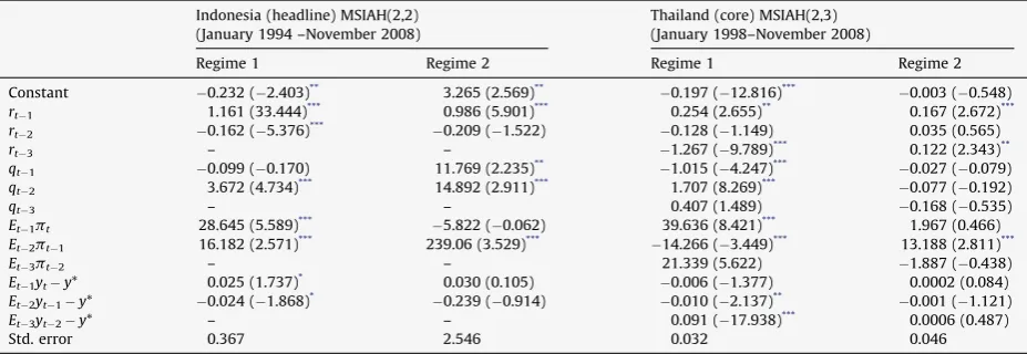
Table 7presents the estimates from the MS-VAR. To incorporate regime shifts in the conditional variance, two and three

states were estimated. Testing was performed with both the normal and thet-distribution, and with different lags based on

the Akaike Information Criteria (AIC). In order to arrive at the most plausible speciﬁcation in describing the conditional

volatility, a bottom-up strategy following Krolzig (1997) was pursued. The starting point is to formally test the null

hypothesis of no regime switch (m= 1) against the alternative of a regime switch (m= 2). If the conventional likelihood ratio

test suggests that the null hypothesis of no regime switching can, indeed, be rejected, we then proceed to test the null

hypothesis of two regimes (m= 2) against the alternative of three regimes (m= 3).25

On the basis of the set of bottom-up testing, the monetary policy reaction functions (Eq.(4)) for the two countries are

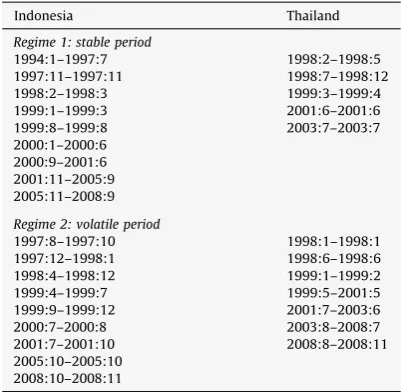
adequately characterized as having at most two regimes (stable (Regime 1) and volatile (Regime 2)) during the period of

observation.26

In general, we find the significant coefficient estimates to have theoretically consistent signs (Table 7). Based on the sizes

of the standard errors and the dates listed, it is clear that Regime 2 is associated predominantly with the periods of economic

turbulences (Table 8). As expected, the early and peak stages of the 1997 ﬁnancial crises, covering the period of the third

quarter of 1997 to late 1999, have predominantly fallen under Regime 2. For the case of Thailand, a large part of the country’s IT period has taken place during the volatile regime, especially since August 2003. In contrast, the IT policy in Indonesia had largely beneﬁted from a relatively stable period (Regime 1). Whilst the breakdowns of the regimes suggest that the management of the policy rate in Thailand has seen a more turbulent period during the recent sub-prime crisis, both countries were in Regime 2 in the immediate aftermath of the closure of the Lehman Brothers in September 2008.

Most importantly, our test results provide adequate evidence that managing inﬂationary expectation has indeed been the focus of the monetary policies of these economies during both stable and volatile regimes. Hence, there has in fact been a credible commitment to the implementation of the IT policy in these two economies. In particular, the commitment of Bank of Thailand to pursue the IT policy has withstood a predominantly turbulent period.

We also ﬁnd that during the stable period (Regime 1), Indonesia and Thailand had adopted a ﬂexible approach to the IT

policy, or what is known as the ITframework.27_{The policy rate has been adjusted accordingly in response to exchange rate}

volatility, inﬂationary expectation, and the expected output gap (Table 7). Interestingly, a greater policy focus has been

Table 7

MS-VAR test results.

Indonesia (headline) MSIAH(2,2) (January 1994 –November 2008)

Thailand (core) MSIAH(2,3) (January 1998–November 2008)

Regime 1 Regime 2 Regime 1 Regime 2

Constant 0.232 (2.403)** _{3.265 (2.569)}**

0.197 (12.816)***

0.003 (0.548) rt1 1.161 (33.444)*** 0.986 (5.901)*** 0.254 (2.655)** 0.167 (2.672)*** rt2 0.162 (5.376)*** 0.209 (1.522) 0.128 (1.149) 0.035 (0.565)

rt3 – – 1.267 (9.789)*** 0.122 (2.343)**

qt1 0.099 (0.170) 11.769 (2.235)** 1.015 (4.247)*** 0.027 (0.079) qt2 3.672 (4.734)*** 14.892 (2.911)*** 1.707 (8.269)*** 0.077 (0.192)

qt3 – – 0.407 (1.489) 0.168 (0.535)

Et1pt 28.645 (5.589)*** 5.822 (0.062) 39.636 (8.421)*** 1.967 (0.466)

Et2pt1 16.182 (2.571)*** 239.06 (3.529)*** 14.266 (3.449)*** 13.188 (2.811)***

Et3pt2 – – 21.339 (5.622) 1.887 (0.438)

Et1yty* 0.025 (1.737)* 0.030 (0.105) 0.006 (1.377) 0.0002 (0.084)

Et2yt1y* 0.024 (1.868)* 0.239 (0.914) 0.010 (2.137)** 0.001 (1.121)

Et3yt2y* – – 0.091 (17.938)*** 0.0006 (0.487)

Std. error 0.367 2.546 0.032 0.046

Note: The numbers inside () are thet-statistics.t-Test critical values: at 1% = 2.66; at 5% = 2.00 and at 10% = 1.67. ***

Signiﬁcance at 1%. **

Signiﬁcance at 5%. *

Signiﬁcance at 10%.

24

Here again, we employ four unit-root tests: the BLS; the standard Augmented Dickey Fuller (ADF) test; the Phillip–Perron test; and the KPSS test. For the sake of brevity, we do not report the results in the paper.

25

A word of caution is necessary in interpreting this result. In Markov-switching models, the usual regularity conditions justifying the use of classical tests such as the likelihood ratio test are violated. This is because, under the null hypothesis of only one state, the transition probabilities are not identiﬁed, implying that the sample likelihood function is ﬂat with respect to these parameters. As inHamilton and Susmel (1994), the likelihood ratio test results mentioned here should be treated more as a descriptive summary than formal statistical tests. The likelihood ratio test statistics can be made available upon request.

26

We also apply the LR statistics to select the optimal MS-VAR model, i.e. to test the null of MSH and MSIH model against the alternative of the more unrestricted MSIAH model.

(15)

placed on inflationary expectation during the turbulent period. The test results seem to suggest that during the volatile period, the output gap did not significantly influence the interest rate policy of both Bank Indonesia and Bank of Thailand. In

the case of Thailand, the monetary authority shifted to a full ITrulefrom the ITframeworkduring Regime 2. As for Indonesia,

managing exchange rate volatility continued to be one of the objectives of interest rate policy in addition to anchoring inflationary expectations. This finding on the importance of managing exchange rate volatility supports the official

statement of Bank Indonesia on its implementation of the IT policy framework (Alamsyah et al., 2001).

In summary, a credible and flexible commitment to the IT framework is evident in Indonesia and also Thailand. Both Bank Indonesia and Bank of Thailand pursued a forward looking policy to manage prices, exchange rate volatilities, and output gaps. The countries’ monetary authorities were steadfast in anchoring inflationary expectations, especially during Regime 2. During the more stable period, IT policy adjustment was aimed at balancing inflation, exchange rate volatilities, and output

stabilities (Table 7).

5. Concluding remarks

A series of initiatives have been proposed and implemented by the Asian governments to avoid a repeat of the 1997 financial crises. The deepening of bond markets is another important step taken to reduce reliance on bank financing. Recent years have also seen impressive growth in the net foreign asset holdings of the Asian economies. In addition to the strengthening of the key financial institutions and reducing potential vulnerabilities of the financial sector, there is a growing general consensus among policy makers and academics that consistent macroeconomic policy frameworks must be in place. In the pursuit of a credible anchor for monetary policy, maintaining price stability, either as an explicit or implicit nominal anchor of a monetary policy framework, has clearly gained popularity over the last decade. Prior to the outbreak of the 1997 East Asian financial crises, none of the Asian economies adopted the IT policy. Indeed, only a total of five developed economies officially announced their inflation targets before 1997. In contrast, by the end of 2006, 24 economies have inflation targeting as the official policy objective of their monetary authorities, with more than half being from emerging markets.

Our paper has examined the implementation and the performance of the IT policy in Indonesia and Thailand. We conducted in-depth analyses on the pass-through effects, both for non-tradable and tradable goods prices in the local economies. In addition, the Markov-switching approach is employed to test for the shift in the monetary policy rule of monetary authorities during the pre-and post-IT periods. In general, these economies have seen their inﬂation rates fall during the post-IT period. The pass-through effects in these economies have, in general, declined considerably except for tradable goods prices of Indonesia. Furthermore, we ﬁnd robust evidence of the credible implementation of IT policy in these

two economies during both stable and volatile periods. While Indonesia continued with itsﬂexible IT framework, Thailand

shifted to astrict IT ruleduring the turbulent period.

References

Aizenman, J., Hutchison, M., & Noy, I. (2008).Inﬂation targeting and real exchange rates in emerging marketsNBER working paper, no. 14561.

Alamsyah, H., Joseph, C., Agung, J., & Zulverdy, D. (2001). Towards implementation of inﬂation targeting in Indonesia.Bulletin of Indonesian Economic Studies, 37(3), 309–324.

Table 8

MS-VAR stable and volatile regimes.

Indonesia Thailand

Regime 1: stable period

1994:1–1997:7 1998:2–1998:5

1997:11–1997:11 1998:7–1998:12

1998:2–1998:3 1999:3–1999:4

1999:1–1999:3 2001:6–2001:6

1999:8–1999:8 2003:7–2003:7

2000:1–2000:6 2000:9–2001:6 2001:11–2005:9 2005:11–2008:9

Regime 2: volatile period

1997:8–1997:10 1998:1–1998:1 1997:12–1998:1 1998:6–1998:6 1998:4–1998:12 1999:1–1999:2

1999:4–1999:7 1999:5–2001:5

1999:9–1999:12 2001:7–2003:6

2000:7–2000:8 2003:8–2008:7

2001:7–2001:10 2008:8–2008:11 2005:10–2005:10

2008:10–2008:11

(16)

Banerjee, A., Lumsdaine, R. L., & Stock, J. H. (1992). Recursive and sequential tests of the unit-root test and trend break hypotheses: Theory and international evidence.Journal of Business and Economic Statistics, 10, 271–287.

Bernanke, B., & Mishkin, F. S. (2007). Inﬂation targeting: A new framework for monetary policy? In Mishkin (Ed.),Monetary policy strategy. Cambridge, MA, USA: The MIT Press.

BIS. (2005).75th annual report (Basel).

Boediono. (1998). Merenungkan Kembali Transmisi Kebijakan Moneter di Indonesia [Revisiting the monetary transmission mechanism in Indonesia].Buletin Ekonomi Moneter dan Perbankan, 1(1), 1–4.

Bryan, M. F., & Cecchetti, S. G. (1995). The seasonality of inflation.Economic Review of the Federal Reserve Bank of Cleveland, 31, 12–23 Quarter 2. Campa, J. M., & Goldberg, L. S. (2002, May).Exchange rate pass-through into import prices: A macro or micro phenomenon?NBER working paper, no. 8934. Cecchetti, S. G. (1997). Measuring short-run inflation for central bankers.Economic Review of the Federal Reserve Bank of St. Louis, 79(May/June), 143–156. Cecchetti, S. G., & Ehrmann, M. (1999, December).Does inflation targeting increase output volatility? An international comparison of policy makers’ preferences and

outcomesNBER working paper, no. 7426.

Chadha, J. S., Lucio, S., & Valente, G. (2004). Monetary policy rules, asset prices, and exchange rates.IMF Staff Papers 51(3).

Charoenseang, J., & Manakit, P. (2007). Thai monetary policy transmission in an inﬂation targeting era.Journal of Asian Economics, 18, 144–157. Clarida, R. (2001). The empirics of monetary policy rules in open economies.International Journal of Finance and Economics, 6(4), 315–323. Clarida, R., Gali, J., & Gertler, M. (1998). Monetary policy rules in practice: Some international evidence.European Economic Review, 42(6), 315–323. Cogley, T. (2002, February). A simple adaptive measure of core inﬂation.Journal of Money, Credit, and Banking, 34(1), 94–113.

Corbo, V., Landerretche, O., & Schmidt-Hebbel, K. (2001). Assessing inﬂation targeting after a decade of world experience.International Journal of Finance and Economics, 6, 343–368.

Edwards, S. (2006, April).The relationship between exchange rates and inﬂation targeting revisitedNBER working paper, no. 12163.

Frankel, J., Parsley, D., & Wei, S. J. (2005).Slow pass-through around the world: A new import for developing countries?NBER working paper, no. 11199. Gagnon, J. E., & Ihrig, J. (2004). Monetary policy and exchange rate pass-through.International Journal of Finance and Economics, 9(4), 315–338. Hamilton, J. D. (1989). A new approach to the economic analysis of nonstationary time series and the business cycle.Econometrica, 57(2), 357–384. Hamilton, J., & Susmel, R. (1994). Autoregressive conditional heteroscedasticity and changes in regime.Journal of Econometrics, 64, 307–333. Hendry, D. F. (1976). The structure of simultaneous equations estimators.Journal of Econometrics, 4, 51–88.

Ho, C., & McCauley, R. N. (2003).Living with ﬂexible exchange rates: Issues and recent experience in inﬂation targeting emerging market economiesBIS working papers, no. 130.

Hodrick, R. J., & Prescott, E. C. (1997, February). Postwar U.S. business cycles: An empirical investigation.Journal of Money, Credit and Banking, 29(1), 1–16. IMF. (2005, September).World economic outlookChapter IV.

Jansen, K. (2001). Thailand, ﬁnancial crisis and monetary policy.Journal of the Asia Paciﬁc Economy, 6(1), 124–152.

Kastner, S. L., & Kim, S. Y. (2008). Why the rush to bilateral free trade agreements in Asia-Paciﬁc? Presented at theinternational studies association annual meeting. Krolzig, H.-M. (1997).Markov switching vector autoregression. Berlin: Springer-Verlag.

Kubo, A. (2008). Macroeconomic impact of monetary policy shocks: Evidence from recent experience in Thailand.Journal of Asian Economics, 19, 83–91. McCauley, R. N. (2006). Core versus headline inﬂation targeting in Thailand. Paper presented inBank of Thailand’s international symposium on Challenges