Watershed-scale impacts of stormwater green infrastructure on
hydrology, nutrient
fl
uxes, and combined sewer over
fl
ows in the
mid-Atlantic region
Michael J. Pennino
a,⁎
, Rob I. McDonald
b, Peter R. Jaffe
a aDepartment of Civil and Environmental Engineering, Princeton University, Princeton, NJ, USA bGlobal Cities Program, The Nature Conservancy, Arlington, VA, USA
H I G H L I G H T S
•Cumulative impacts of multiple stormwater green infrastructure sys-tems
•Statistical analyses on SGI, hydrologic, and water quality data were conducted. •Hydrologicflashiness is lower in water-sheds with stormwater green infra-structure.
•Stream nitrogen loads are lower in wa-tersheds with stormwater green infra-structure.
G R A P H I C A L A B S T R A C T
Impact of stormwater green infrastructure (SGI) on hydrology and nitrogen export. The % values represent the percent change between low and high SGI.
a b s t r a c t
a r t i c l e
i n f o
Article history:
Received 3 March 2016
Received in revised form 14 May 2016 Accepted 15 May 2016
Available online 31 May 2016
Editor: Jay Gan
Stormwater green infrastructure (SGI), including rain gardens, detention ponds, bioswales, and green roofs, is being implemented in cities across the globe to reduceflooding, combined sewer overflows, and pollutant trans-port to streams and rivers. Despite the increasing use of urban SGI, few studies have quantified the cumulative effects of multiple SGI projects on hydrology and water quality at the watershed scale. To assess the effects of SGI, Washington, DC, Montgomery County, MD, and Baltimore County, MD, were selected based on the availabil-ity of data on SGI, water qualavailabil-ity, and streamflow. The cumulative impact of SGI was evaluated over space and time by comparing watersheds with and without SGI, and by assessing how long-term changes in SGI impact hy-drologic and water quality metrics over time. Most Mid-Atlantic municipalities have a goal of achieving 10–20% of the landscape drain runoff through SGI by 2030. Of these areas, Washington, DC currently has the greatest amount of SGI (12.7% of the landscape drained through SGI), while Baltimore County has the lowest (7.9%). When controlling for watersheds size and percent impervious surface cover, watersheds with greater amounts of SGI have lessflashy hydrology, with 44% lower peak runoff, 26% less frequent runoff events, and 26% less var-iable runoff. Watersheds with more SGI also show 44% less NO3−and 48% less total nitrogen exports compared to watersheds with minimal SGI. There was no significant reduction in phosphorus exports or combined sewer overflows in watersheds with greater SGI. When comparing individual watersheds over time, increases in SGI
Keywords:
Urban
Stormwater management Hydrologicflashiness Nitrogen exports Phosphorus exports Water quality
⁎ Corresponding author at: US Environmental Protection Agency, National Health and Environmental Effects Research Laboratory, Western Ecology Division, Corvallis, OR, USA.
E-mail address:[email protected](M.J. Pennino).
http://dx.doi.org/10.1016/j.scitotenv.2016.05.101
0048-9697/© 2016 The Authors. Published by Elsevier B.V. This is an open access article under the CC BY-NC-ND license (http://creativecommons.org/licenses/by-nc-nd/4.0/). Contents lists available atScienceDirect
Science of the Total Environment
corresponded to non-significant reductions in hydrologicflashiness compared to watersheds with no change in SGI. While the implementation of SGI is somewhat in its infancy in some regions, cities are beginning to have a scale of SGI where there are statistically significant differences in hydrologic patterns and water quality.
© 2016 The Authors. Published by Elsevier B.V. This is an open access article under the CC BY-NC-ND license (http://creativecommons.org/licenses/by-nc-nd/4.0/).
1. Introduction
In urban areas the connection of impervious surfaces (i.e. roads, parking lots and roofs) to traditional grey infrastructure (i.e. storm drains, storm sewers and combined sewer systems) was originally intended to convey stormwater runoff and reduceflooding (American Rivers, 2016; Dunne and Leopold, 1978; Wang et al., 2013). However, these traditional stormwater systems are known to result in the erosion of waterways, water pollution, degradation of downstream ecosystems during wet weather events, and localizedflooding (De Sousa et al., 2012; Leopold, 1968; Paul and Meyer, 2001; Walsh et al., 2005). Also, runoff often contains pollutants, such as nutrients that deposit on sur-faces (US EPA, 2009). When impervious surface area and runoff is high,flooding and CSOs can result (De Sousa et al., 2012; Paul and Meyer, 2001). While there are grey infrastructure solutions, many cities are looking to use green infrastructure as a way to help mitigate prob-lems with their stormwater system. As a result, stormwater green infra-structure (SGI), which includes rain gardens, detention ponds, bioswales, green roofs and more, is being implemented throughout major cities across the United States, to help mitigateflooding, water quality, and combined sewer overflows (CSOs) problems, resulting from traditional grey infrastructure (US EPA, 2015a).
Most municipalities across the U.S. have incorporated SGI into their sustainability plans (e.g.NYC DEP, 2013; Sustainable DC, 2011) and many cities have a consent decree issued by the EPA, where they are re-quired to control stormwater pollution and CSOs. Cities often use SGI as a major part of their mitigation strategy (US EPA, 2015b). SGI is being implemented nationwide, from New York (NYC DEP, 2013) to Cleveland (Sustainable Cleveland, 2013) to Chicago (City of Chicago, 2014) to Se-attle (Seattle Public Utilities, 2015). In fact, millions of dollars have been spent in each city on SGI (e.g.NYC DEP, 2013). Cities typically have a goal of using SGI to capture 10–20% of the drainage area across the landscape (e.g.NYC DEP, 2013; Sustainable DC, 2011).
Yet, even though a lot of cities are implementing SGI and have been implementing SGI for over a decade, there have been very few studies on whether there are detectable impacts on hydrology, water quality, and CSOs, at the city or regional scale (Hale et al., 2015; Meierdiercks et al., 2010; Smucker and Detenbeck, 2014). Most research has focused on the site-level impacts of SGI on water quality and quantity (e.g. Barrett, 2008; Bettez and Groffman, 2012; Bratieres et al., 2008; Davis, 2007). The studies that do look at watershed-scale have only compared two paired watersheds (Burnsville, 2006; Dietz and Clausen, 2008; Hager et al., 2013; Roy et al., 2008; Yang and Li, 2013). These studies have generally found there to be positive impacts on hydrology, nutri-ent loading, and stream biota (Smucker and Detenbeck, 2014), though none of these studies are at the city or regional scale. Also, most studies on the watershed-scale impacts of SGI are based on models (e.g. Emerson et al., 2005; Liu et al., 2015). This current study is, to our knowledge, thefirst to compile publicly available data to empirically as-sess the cumulative impacts of multiple SGI projects on hydrology, water quality, and combined sewer overflows at the watershed scale and across multiple watersheds over an entire region.
2. Methods
2.1. Study site selection and data sources
Three areas were selected in the Mid-Atlantic region of the United States: Baltimore County, MD, Montgomery County, MD, and
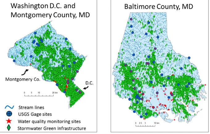
Washington, DC (referred to as DC herein after). These locations were chosen based on their geographic proximity and the abundance of avail-able data (Note that there was no SGI data availavail-able for Baltimore City, but some of the watershed in the analysis overlap Baltimore City). From each region public and private data was compiled on the locations of SGI facilities, streamflow data, long-term stream chemistry, and for DC only long-term combined sewer overflow data was obtained (Fig. 1, Fig S1). For hydrologic and water quality analyses, watersheds were selected based on the presence of a USGS stream gage and long-term water quality data. All watersheds selected had a USGS stream gage, but not all watersheds had available water quality data (Table S1). Watershed sizes ranged from 0.5 to 34.3 km2with a median
area of 6 km2(Table 1). For CSO analysis, individual sewersheds that drain to each CSO were selected. The sewershed size ranged from 12 m2to 5.6 km2, with a median area of 0.2 km2(Fig. S1,Table 1). All
sites in this study, are within the Piedmont physiographic region, and have had approximately the same average annual rainfall since 1984 of 39.4 in. in DC and 40.8 in. in Baltimore (NOAA, 2014).
Stormwater green infrastructure data was provided as GIS point layers from each municipality. For DC, the SGI data was obtained from DC OCTO (data.octo.dc.gov) and for Montgomery County, MD, SGI data was obtained from the Montgomery County Department of Envi-ronmental Protection (MCDEP, 2015). For Baltimore County, MD, the Baltimore County Department of Environment and Sustainability pro-vided a link to their SGI data on their National Pollutant Discharge Elim-ination System (NPDES) MS4 Report page, under the heading NPDES Permit Data (BCDES, 2015).
For each of the three regions, GIS data on the locations of stream gage sites came from the USGS (USGS, 2015). For each USGS stream gage, data on instantaneous streamflow was obtained from USGS Water Data for the Nation (waterdata.usgs.gov/nwis). Instantaneous flow ranged from 1 min intervalflow data to 15 min intervalflow data, in cubic feet per second (cfs). The water quality parameters (nutri-ents) used in this study were nitrate (NO3−), total nitrogen (TN),
phos-phate (PO4−3), and total phosphorus (TP). Long-term water quality
data was obtained from various sources, including the National Water Quality Monitoring Council, which includes data from the EPA and USGS (NWQMC, 2015), the Baltimore Ecosystem Study Long-term Eco-logical Research site (BES, 2015), and Clean Water Baltimore Water Sampling Program (CWB, 2015). CSO data was obtained separately. For DC, CSO data was obtained from DC Water and Sewer Authority's Combined Sewer System Quarterly Reports (DC WASA, 2015) and DC Atlas Plus (DC Atlas Plus, 2015).
GIS data on regional boundaries, hydrography, digital elevation model (DEM) data were obtained from the NRCS Data Gateway (NRCS, 2015). Land use and impervious surface cover was obtained from the Multi-Resolution Land Characteristics Consortium National Land Cover Database (NLCD) for 2001, 2006 and 2011 (MRLC, 2015).
2.2. Hydrologic metrics
Hydrologic metrics were calculated using instantaneous discharge. Metrics consisted of the following variables, also shown in supporting information Table S2: (1) average annual peak runoff (mean of runoff value from each hydrograph peak) (similar toSmith et al., 2013), (2) av-erage annual baseflow (estimated after removing periods of surface runoff or hydrographs from discharge data), (3) high-flow event fre-quency (frefre-quency of peaks above 3 × monthly medianflow), called
“peak frequency”from this point on (Utz et al., 2011), (4) volume-to-1045
peak ratio (hydrograph volume divided by peakflow discharge) (Smith et al., 2013), (5) hydrograph duration (time from start to end of hydrograph) (Kennard et al., 2010; Olden and Poff, 2003), and (6) coef-ficient of variation in runoff (Kennard et al., 2010). These metrics were chosen to provide a sense of how variability in urbanization and water-shed management affect typical stormflow characteristics and the vari-ability in hydrologic response to storm events. These variables are also termed as metrics of hydrologicflashiness, which is characterized by flow events with higher peaks, quicker time to peak, and shorter falling limbs (Konrad et al., 2005; Loperfido et al., 2014; Meierdiercks et al., 2010; Smith et al., 2013; Sudduth et al., 2011; Walsh et al., 2005). All hy-drologic metrics were estimated using MATLAB 8.3.0 (MATLAB and Sta-tistics Toolbox Release R2014a Student) and despite the different time intervals for hydrology data it was found that overall there is only a 5.1 ± 3.1% difference when using 1 vs. 15 min interval data or 5 vs. 15 min interval data (see Table S3).
2.3. Nutrient exports
Routinely sampled concentration data, mean daily discharge, and the USGS FORTRAN program LOADEST (Runkel et al., 2004) were used to calculate the annual loads of all stream chemistry variables (NO3−,
TN, PO4−3, and TP) at each site. LOADEST uses a multiple parameter
re-gression model that accounts for bias, data censoring, and non-normal-ity to minimize difficulties in load estimation (Qian et al., 2007). Load is estimated using one of three statistical approaches: Adjusted Maximum Likelihood Estimation (AMLE), Maximum Likelihood Estimation (MLE), and Least Absolute Deviation (LAD). AMLE was chosen when the cali-bration model errors (residuals) were normally distributed, while LAD was chosen when residuals were not normally distributed(Runkel et
al., 2004). Annual nutrient export (mass/area/year) was calculated by summing daily loads (mass/day) for each year and dividing by water-shed area. Through analyses of model residuals and a comparison of the observed and estimated loads, any constituents found to have bias in the LOADEST output (Runkel, 2013) were excluded from the analysis. The routine sampling for the majority of stream sites was able to obtain a range of streamflow, overlapping many annual storm events (Fig. S2), though the highest storm events were likely not captured due to the sampling frequency (Table S1) and safety concerns. As a result, the an-nual loads estimated from this dataset may not fully estimate the stormflow contribution. However, because all sites are within the same region and receive relatively the same rainfall during storm events, we believe the relative annual exports estimated for the sites are comparable and it is appropriate to draw conclusions among the study sites. Additionally, SGI was expected to have an impact on nutri-ent exports even during baseflow conditions, as SGI can influence bio-geochemical processing (Bettez and Groffman, 2012; Newcomer Johnson et al., 2014) and the amount of infiltration and groundwater re-charge within a watershed (Freeborn et al., 2012; Newcomer et al., 2014; Shafique and Kim, 2015). Additionally,flow normalized concen-trations were estimated using EGRET package in R (Hirsch and De Cicco, 2015).
2.4. Data organization and analysis
The SGI data included estimates for the drainage area for each SGI fa-cility, which is the area of land that drains to a particular SGI facility. Bal-timore County and Montgomery County GIS data included polygon shapefiles to represent the drainage area for each SGI facility, while DC only provided a number for each drainage area estimate, but no polygon Fig. 1.The 3 Mid-Atlantic cities where data on stormwater green infrastructure (green dots), USGS gages (blue dots), and water quality monitoring sites (red stars).
Table 1
Ranges and averages (±standard errors) for the watershed and sewershed area, %ISC, and %SGI.
N Low SGI Sites
N High SGI Sites
Shed Area Range (km2)
Mean Area (km2)
Median Area (km2)
% ISC Range
Mean % ISC
Median % ISC
% SGI Range
Mean % SGI
Median % SGI
Hydrology Data
6 19 0.5–34.3 8.1 ± 1.6 6.0 13.7–53.0 29.9 ± 2.2 30 0–58 22.7 ± 3.7 22
Water Quality Data
5 11 0.5–34.3 10.5 ± 2.6 9.0 13.7–53.0 29.4 ± 4.1 22 0–58 18.6 ± 6.3 15
DC CSO 23 20 0–5.6 0.6 ± 0.2 0.2 17.7–89 61.7 ± 2.9 67 0–62.1 11.9 ± 2.0 9.6
file. Due to the differences in SGI drainage area data, Baltimore County and Montgomery County were only used for the hydrologic and water quality analyses, while the DC SGI data was only used for the CSO anal-ysis. Using ArcGIS and the drainage area polygons, the percent SGI in each watershed was calculated by clipping the polygons within each watershed and then dividing the total polygon area by the watershed area. And for DC the percent SGI in each watershed was calculated based on summing the drainage area for each SGI facility within the wa-tershed and then dividing this value by the area of the wawa-tershed. For DC most of the drainage areas attributed to each SGI facility were given, but for those that were not given (about 17% of the ~2700 SGI fa-cilities), average drainage areas were given based on specific SGI type found in DC (i.e. rain gardens, detention ponds, infiltration trench, etc.). Additionally, to test the effect of different SGI types in Baltimore County, Montgomery Counties, and DC, we calculated the percentage SGI for each major SGI type: detention ponds (DP), shallow marsh (SM), wet pond (WP), sandfilter (SF), infiltration trend/basin (IT), bioretention (BR), and swales (SW), and included these % SGI values in Table S1 in supporting information. For CSO data we also added an SGI category that includes catch basins, stormceptors, stormfilters and baysavers (called CB).
Sites used in the hydrologic and water quality analyses were chosen to have an areab40 km2, to reduce the range of watershed sizes and also help to minimize the impact of larger watersheds, which typically have lessflashy hydrology (Brezonik and Stadelmann, 2002; Galster et al., 2006). Watersheds were also chosen to have an impervious area N10%, to help exclude non-urban or forested sites from the analysis, which may obscured the data due to these sites having low % SGI, but also lowflashiness and nutrient exports (O'Driscoll et al., 2010; Smith et al., 2013). The 10% imperviousness cutoff was also chosen because levels of imperviousnessN10% have been shown to have negative im-pacts on aquatic ecosystems (e.g.Beach, 2001; Booth, 1991; Klein, 1979). Due to the removal of sites with areas N40 km2 and with ISCb10%, out of a possible 50 watersheds in Baltimore County and Montgomery County, 23 were used for the hydrologic analysis and 13 were used for water quality analysis (see Tables S1,1, S4). Compared to all possible watersheds, the average and median watershed areas were lower for this study, while the ISC was higher and the %SGI was more similar (Tables 1and S4).
2.5. Statistical analysis
To assess whether there currently is a significant effect of SGI on hy-drology, water quality, and CSO metrics, multi-linear regression was used to look at the effect of SGI (for total SGI and for each SGI type sep-arately), while controlling for the effect of impervious surface cover and watershed size. Using the same data, ANOVA was also used to compare watersheds with little or no SGI, called“low SGI”(b5% SGI) to water-sheds withN5% SGI, called“high SGI,”while accounting for the effect of impervious surface cover and watershed size. Both analyses were done using the mean annual value for each variable, averaged for mul-tiple years (2011, 2012, 2013 for hydrology and water quality data and 2011, 2012, 2013, 2014 for CSO data). ISC and watershed size were controlled by including these variables as cofactors in the multi-linear or ANOVA models, which allowed individualp-values to be ob-tained for each variable. For the ANOVAs we conducted a sensitivity analysis to test for the impact of changing the % SGI cutoff for low vs. high SGI from being 3%, 5%, or 10%. We also tested the impact of remov-ing outliers in the nutrient export multi-linear regression analysis. To assess whether there are significant trends over time, long-term data on SGI, hydrology, water quality, and CSO metrics averaged for each year from 2005 to 2014 were used to assess whether any change in these metrics can be attributed to an increase in SGI over time, com-pared to“control”watersheds where there was no change in SGI over that time period. ANOVA was then used to compare the percent change in each metric for sites with no change over time in SGIvs. sites with
N5% increase in SGI over time for hydrology and CSO data or 1-6% in-crease in SGI for water quality data, while accounting for the effect of impervious surface cover and watershed size. The 1 or 5% increase in SGI cutoff was chosen due to the small sample size and lack of sites with a large increase in SGI over time. For both multi-linear regression and ANOVA, to test the assumption of normal distribution and homoge-neous model residuals, the Shapiro–Wilk test (Royston, 1982) and the normal Q–Q plot were performed. The hydro, water quality, or CSO met-rics that did not meet those assumptions were either log or square root transformed prior to statistical analysis. All statistical analysis was done in R (R Development Core Team, 2015) using the aov function for ANOVA and the lm function for multi-linear regression. For testing nor-mality assumptions of the ANOVA and multi-linear regressions, the shapiro.test, qqnorm, and qqline functions were used.
3. Results and discussion
3.1. Stormwater green infrastructure comparison across study areas
The municipalities in this study have set a goal to, within the next 15 years, have 15–20% of the land area to have runoffflow through SGI (Fig. 2). Regions like Baltimore County and DC, which have been implementing SGI for over a decade, currently have approximately 10% of their total landscape managed by SGI (Fig. 2). Of the areas in this study DC currently has the greatest level of landscape drained through SGI (12.7%), while Baltimore County has the lowest (7.9%,Fig. 2).
3.2. Stormwater green infrastructure impacts hydrology
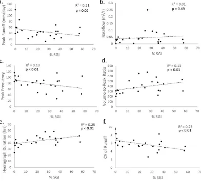
For watersheds in Baltimore County and Montgomery County, re-sults from ANOVA analysis show that SGI has a significant effect on hy-drology at the watershed scale, where watersheds withN10% SGI show a 26 to 44% reduction in hydrologicflashiness metrics compared to wa-tersheds without SGI (Table 2). Based on multi-linear regression, with % SGI as a continuous variable and ISC and watershed size as covariates, all of the hydrology metrics showed a significant relationship with % SGI (pb0.05), except baseflow (Figs. 3, S3).
When using ANOVA with SGI as a categorical variable (low SGIvs. high SGI), and after controlling for impervious area and watershed size, watersheds with high % SGI have lower peak runoff, less frequent peaks, longer hydrograph duration, lower CV for runoff, and a higher volume-to-peak ratio (pb0.05,Fig. 4a). SGI showed no significant effect on baseflow (Fig. 4a). This indicates that as the percent of stormwater green infrastructure increases for watersheds, the magnitude, frequen-cy, duration, variability orflashiness of stormwater events is reduced (Fig. 3). This is encouraging for watershed managers who need to re-duce the potential forflooding and urban stream erosion due to runoff
Fig. 2.Comparison of existing SGI levels and each municipality's goal level of SGI. 1047
from impervious surface areas. It was also found based on the sensitivity analysis that there is no difference on the hydrology results when a 3%, 5%, or 10% SGI cutoff (for low SGIvs. high SGI) is used (Table S5).
Using the different SGI types we conducted a multi-linear regression analysis using each SGI type separately and using watershed area and impervious surface cover as co-variates. Wefind that some of the met-rics are significantly correlated with the specific SGI types (Table S6). For the hydrology data, peak runoff is significantly correlated with de-tention ponds (DP) and shallow marshes (SM), but no other SGI type, which is not surprising because detention ponds and marshes are typi-cally designed to retain water temporarily from impervious surfaces and thus reduce peakflow volumes (Freeborn et al., 2012; Newcomer et al., 2014; Shafique and Kim, 2015). Peak frequency is significantly correlated with SF, IT, and BR (Table S6). Volume-to-peak ratio is signif-icantly correlated with sandfilters (SF) and infiltration trenches (IT) (Table S6). Hydrograph duration is significantly correlated with SM, SF, and IT (Table S6). CV of runoff is correlated with all but DP and WP (Table S6). Baseflow was only correlated with IT (Table S6). WP had no sig relationships (Table S6). Overall, SF and IT appear to have the greatest relationships with the hydrologic metrics, possibly due to prev-alence of these SGI types (Table S1) and their ability to increase infi ltra-tion (Freeborn et al., 2012; Newcomer et al., 2014; Shafique and Kim, 2015) more than the other SGI types.
When looking at long-term trends in SGI and hydrology, increases in SGI (2005–2014) were not associated with significant impacts on water quantity, however, a number of hydrologic metrics show promising trends, which would be beneficial to stormwater management (Fig. 4b). Over time the control watersheds (with no change in SGI) showed
an increase in peak runoff and the CV of runoff, while watersheds with N5% increases in SGI over time showed little or no change in these met-rics (p= 0.24 andp= 0.47, respectively). The volume-to-peak ratio showed a slight decrease for control watersheds compared to sites with increasing SGI (p= 0.12). This all indicates that watersheds with-out SGI may be becoming slightlyflashier in hydrology, while the water-sheds with increases in SGI show little change in hydrologicflashiness metrics. Yet the data is highly variable, with peak frequency, mean baseflow, and hydrograph duration, showing no difference between control site and watersheds with increases in SGI (Fig. 4b). The variabil-ity was likely not due to changes in impervious surface cover over time because all sites had less than a 4% increase in % ISC from 2001 to 2011. This variability may be due to increases in climate variabilities, as stud-ies show that the Potomac and the Susquehanna rivers, both in the Bal-timore County and DC regions, have become more variable, with greater hydrologic extremes over the past 30 or more years (Kaushal et al., 2010; Lee, 2015). Still, due to the promising trends in the data, future in-creases in SGI may show more significant differences between control sites and watersheds with greater increases in SGI.
scale, when the % SGI is larger than 3 or 5%, which indicates that this may also be the case in larger watersheds with similar % SGI. Also, with further research, it may be possible to show how the hydrologic impacts found only at the site or small watershed level (Davis, 2008; Hunt et al., 2006; Li et al., 2009) can be scaled up to intermediate or larg-er watlarg-ershed levels. Increasing the SGI in a watlarg-ershed effectually is re-ducing the connected impervious surface area and increasing the ability to intercept and detain rainwater before it enters stream chan-nels and also increase the infiltration of rain water into the soil
(Freeborn et al., 2012; Newcomer et al., 2014; US EPA, 2015a). This study also supports how stormwater management, if used properly across a watershed, can be essential for protecting stream ecosystems fromflashy hydrology (Walsh et al., 2016). And with the potential for climate change to increase the frequency and magnitude of hydrologic events, SGI systems have the potential to mitigate these impacts (Hale et al., 2016).
3.3. Stormwater green infrastructure impacts nitrogen exports
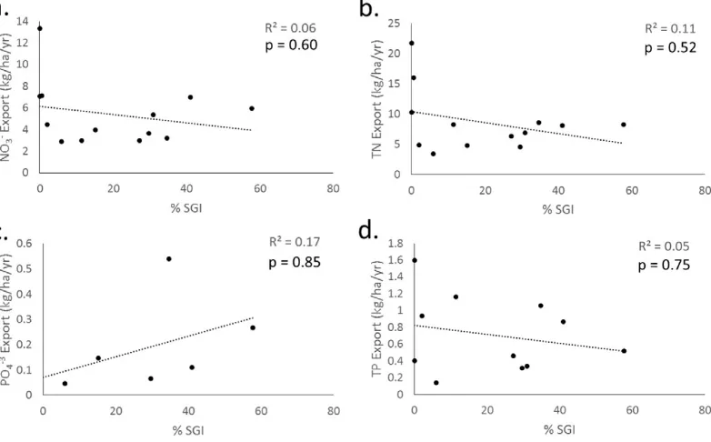
When comparing the level of stormwater green infrastructure in watersheds with the export of nutrients from each watershed spatially across Montgomery County and Baltimore County regions there is a slightly significant effect of SGI on nutrient exports depending on the statistical technique used (Figs. 5 and 6). When using multi-linear re-gression, while controlling for the effect of ISC and watershed size, there is a slight decreasing trend in N and P exports with increasing % SGI (Figs. 5, S4,p= 0.60 and 0.52 for NO3−and TN, respectively and p= 0.85 and 0.75, for PO4−3and TP, respectively). The lack of a more
sig-nificant downward trend for NO3−, TN, PO4-3, and TP may be due
primar-ily to the small sample size, but also to variability in the data. There are a number of factors that likely influence the variability in nutrient exports among watersheds, such as the amount of home lawn care fertilizer use (Zhou et al., 2008), legacy effects of past land use being agriculture (Chen et al., 2015; Van Meter and Basu, 2015) or of potential leaks from sanitary sewers in watersheds with high SGI (Kaushal et al., 2011). In fact, based on NLCD data which shows the % developed open space land (which is mostly vegetation in the form of lawn grasses), many of the sites with higher nutrient exports also have higher lawns areas (Zhou et al., 2008). This is also confirmed by previous studies con-ducted in Baltimore showing that lawns can be significant sources of N to receiving waters (Groffman et al., 2004; Groffman et al., 2009).
When assessing the impact of each different SGI type, the nutrient data is not significantly correlated with any of the individual SGI types, however, for NO3−, SF and IT have lowestp-values, for TN, SM
and BR have lowestp-values, and for TP, IT has lowestp-values (Table S6). The bioretention and shallow marsh systems are known to have higher denitrification rates (Bettez and Groffman, 2012; Davis, 2007) and there may also be high nutrient retention and removal in sand Fig. 4.a) Comparison of average (for years 2011–2013) hydrologic metrics for watersheds
with (N5% SGI) and watersheds without stormwater green infrastructure (b5% SGI) and b) Comparison of % change in hydrologic metric for watersheds with no change in SGI and sites withN5% change in SGI over a 10 year period. Panel A:N= 6 for low SGI andN= 19 for high SGI sites, for all hydrology metrics. Panel B:N= 9 for control sites andN= 5 for sites with increases in SGI. Error bars are standard errors of the mean.
Fig. 5.Effect of stormwater green infrastructure (SGI) on a) NO3−, b) TN, c) PO43−, and d) TP annual exports. Each point represents average annual nutrient export (for years 2011–2013) for each watershed in this study.
1049
filters and infiltration trenches if they are clogged and thus can support standing water and anoxic conditions for denitrification (Chazarenc and Merlin, 2005; Starzec et al., 2005; Torrens et al., 2009). The SGI types with greater retention and infiltration of runoff (which is typical for SF, IT, and SM compared to the smaller BR and SW facilities) likely has a large impact on nutrient exports as nutrient export and runoff are strongly correlated (Shields et al., 2008) (see further discussion below). Due to the potential impact of outlier watersheds found at low SGI, the most outlying point was removed and it was found, as expected,
that the regression relationships become less significant for all nutrients (see Table S7). Additionally, when looking at annualflow normalized andflow weighted concentration data for 2013 it is clear that without the one outlier point there is a significant negative trend for NO3−and
TN with increased % SGI (Fig. S5). This suggests that higher levels of SGI in watersheds may help reduce nutrient concentrations in urban streams, as well as nutrient exports, but further research and more data is needed.
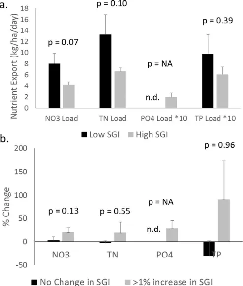
Based on ANOVA results, watersheds with SGI show about 45% lower nitrogen exports compared to watersheds without SGI, (Table 2), which is encouraging for cities who are trying to meet National Pol-lutant Discharge Elimination System (NPDES) stormwater permit re-quirements (US EPA, 2011). When using ANOVA and SGI as a categorical variable (low SGIvs. high SGI), and with ISC and watershed size as covariates, there is a marginally significant effect of SGI on N ex-ports at the watershed scale, but not for phosphorus exex-ports (Fig. 6a). The watersheds with high % SGI, on average, show less NO3−and TN
ex-ports (p= 0.07 andp= 0.1, respectively,Fig. 5a). Due to missing data there were no low SGI watershed values for PO4−3and there was no
sig-nificant difference between watersheds for TP (Fig. 6a,p= NA,p= 0.54, respectively). Based on the sensitivity analysis for the impact of changing the % SGI cutoff for the highvs. low SGI categories, it was found that there is a decrease in thep-values when the %SGI cutoff is changed from 5% to 10% SGI (Table S5). This shows that the impact of SGI on nutrient export is not as robust as the hydrologic data.
The impact of SGI on both hydrology and biogeochemical processing likely plays a role in controlling the nutrient export results. Because SGI measures were found to reduce peak runoff andflashy hydrology it is not surprising that nutrient exports were also reduced. In fact, the sites in this study show that stormflow may play a larger role on total nutrient exports than baseflow as there is a greater percentage of total runoff from storm events (Fig. S6). And as expected, SGI sites have sig-nificantly lower stormflow runoff than sites without SGI (Fig. S6), likely due to the ability of SGI to retain and infiltrate runoff (Freeborn et al., 2012; Newcomer et al., 2014; Shafique and Kim, 2015). Previous studies have shown that there can be a greater contribution to nutrient exports from stormflow events (particularly for P) (e.g.Horowitz, 2009; Shields et al., 2008). However, other studies suggest an equal, if not a greater contribution to nutrient export during baseflow, particularly for N (e.g.Horowitz, 2009; Janke et al., 2014). SGI may also have an impact on nutrient exports during baseflow by reducing the amount of nutri-ents entering through groundwater recharge by intercepting and tem-porarily retaining rainfall runoff from impervious surfaces (Freeborn et al., 2012; Newcomer et al., 2014; Shafique and Kim, 2015) and there-by increasing the biogeochemical removal of nutrients within SGI sites through denitrification, assimilation, or absorption (Bettez and Groffman, 2012; Lucas and Greenway, 2011; Newcomer Johnson et al., 2014). Also, a recent global review and synthesis suggests that certain forms of stream restoration have potential to retain watershed nutrient exports particularly during baseflow, but further evaluation across streamflow is necessary (Newcomer-Johnson et al., 2016). The non-sig-nificant and variable effect of SGI on TP may indicate the SGI sites may not be as effective at removing TP (Alahmady et al., 2013; Hatt et al., 2009), potentially due to older stormwater facilities having less ability to adsorb TP due to saturation of absorption sites (Lucas and Greenway, 2011; Rosenquist et al., 2010). With the number of studies showing how well individual SGI facilities remove N (e.g.Barrett, 2008; Bratieres et al., 2008; Davis, 2007), it is not surprising that these effects can scale up to impact water quality at the watershed scale. How-ever, more watersheds and higher levels of SGI may be necessary to see more significant effects on nutrient exports.
The long-term trends in nutrient exports do not show any significant difference between control watersheds and watershed where % SGI in-creased over time (Fig. 5b). In fact the opposite trend from what is ex-pected is observed, where nutrient exports have increased (though not significantly) more at watersheds with increasing SGI than Fig. 6.(a) Comparison of annual nutrient export for watersheds with (N5% SGI) and
watersheds without stormwater green infrastructure (b5% SGI) and (b) Comparison of % change in nutrient exports for sites with no change in GI and sites withN1% change in SGI over a 10 year period. Panel A: NO3−and TN, low and high SGIN= 4 and 9, respectively, for PO4−3, low and high SGIN= 0 and 6 respectively, and for TP low and high SGI,N= 3 and 8 respectively. Panel B:N= 3 for control sites andN= 6 for SGI sites. Error bars are standard errors of the mean.
Table 2
Hydrology, water quality, and CSO metric descriptions, expected effects of SGI, and percent difference between watersheds with SGI and watersheds without SGI.
Metric Expected effect of SGI % Differencea
Peak runoff (mm/day) Decrease −44 ± 0.9a
Baseflow (m3
/s) Increase 110 ± 1.3
Peak frequency Decrease −26 ± 0.6a
Volume-to-peak ratio (hrs) Increase 133 ± 0.2a
Hydrograph duration (hrs) Increase 27 ± 0.7a
CV of runoff Decrease −26 ± 0.7a
NO3−export (kg/ha/yr) Decrease −44 ± 1.2a
TN export (kg/ha/yr) Decrease −48 ± 1.3a
PO4−3export (kg/ha/yr) Decrease NA
TP export (kg/ha/yr) Decrease −28 ± 2.9
Avg # CSOs Decrease 20 ± 0.8
Total CSO duration (hrs) Decrease 157 ± 4.3
CSO volume (mg) Decrease −20 ± 2.5
% Difference (mean ± 95% confidence interval) is between watersheds with and water-sheds without SGI. Negative % difference means metrics for the waterwater-sheds with SGI are less than for the watersheds without SGI. TN = total nitrogen and TP = total phosphorus.
a
watershed without changes in SGI (Fig. 5b). This again, can likely be at-tributed to small sample size, high variability between watersheds, and also because the increase in SGI was probably too small to have a detect-able effect (ranging between a 1 and 6% increase in SGI over 10 years). In fact, it is somewhat surprising for there to be an increase in nutrient ex-ports over the past 10 years at any of the sites because in the DC, Mont-gomery County, and Baltimore County regions, both total nitrogen and nitrate in atmospheric deposition decline significantly, from 1984 to 2014, with TN declining from 24 to 14 kg and NO3−declining from 16
to 8 kg of deposition per year, based on data from the National Atmo-spheric Deposition Program (nadp.sws.uiuc.edu). Also the % ISC does not increase from 2001 to 2011N1.6% for all the water quality sites. However, one explanation for the increase in nutrient exports over time is that the majority of watershed show that total annual runoff has been increasing over the last 10–20 years (Fig. S7) and as described previously, higher runoff is typically associated with higher exports. An-other possible explanation for the variability and the increase in nutri-ent exports for some watersheds that have higher SGI (particularly the older and more urban watershed) is leaking sanitary sewers, which may be getting worse over time, and there is evidence for this in the Baltimore area (Kaushal et al., 2011; Parr et al., 2016; Pennino et al., 2015). Also, there can be a time lag between decreases in nutrient inputs and the timing of nutrients exported, due to the long retention time of some groundwater reservoirs or the time nutrients spend in vegetation before being demineralized (Galloway et al., 2003; Hamilton, 2012; Hefting et al., 2005). Similarly, another possible infl u-ence on nutrients is the antecedent land use prior to urbanization (Cuffney et al., 2010; Utz et al., 2016). Finally, increases in climate vari-ability can also be a factor in influencing the variability in nutrient ex-ports (Hale et al., 2016; Kaushal et al., 2014; Kaushal et al., 2010; Lee, 2015).
3.4. Stormwater green infrastructure impacts combined sewer overflows
When using multi-linear regression, with ISC and watershed size as covariates, there is no significant relationship between SGI and any of the CSO metrics (frequency, duration, or volume of CSO events, Fig. S8). Similarly, we found that none of the individual SGI types have sig-nificant correlations with the CSO metrics (Table S6). When using ANOVA to compare sewersheds with low SGI to watersheds with high SGI, there are no significant differences and CSO volume is the only met-ric that shows a decrease (though not significant) with high SGI (Fig. S9a,Table 2). . The sensitivity analysis using different %SGI cutoff levels (3%, 5%, and 10%) also showed no difference in CSO results (Table S5). Based on these results, due to the high variability in the data and only one city used in this analysis, there were no significant results.
However, when looking at long-term changes, from 2005 to 2014, there are promising trends for the CSO sewersheds that have had in-creases in SGI compared to sewersheds without SGI (Fig. S9b). The % change in CSO metrics are consistently lower (though not significantly) for sites with increases in SGI (Fig. S9b,p= 0.22, 0.37, and 0.22, for CSO frequency, duration, and volume, respectively). The fact that the CSOs metrics show greater trends towards reductions when SGI increased over time compared to the hydrology and nutrient data may be due to the smaller size of the sewersheds compared to the watersheds, resulting in some sewersheds experiencing up to a 30% increase in SGI over the 10 year period, and thus having a stronger impact on CSOs in those sewersheds. Yet, the lack of significant differences between sewersheds with increases in SGI and sewersheds without is likely due to the large variability among sewersheds. However, there is still a 60 to 70% probability (based on thep-values) that sites with in-creasing SGI overtime have reduced CSOs compared to control sites (Fig. S9b).
Combined sewer overflows are a major problem in cities that have combined stormwater and sewer systems (De Sousa et al., 2012). By intercepting and thus reducing the amount of water entering
stormdrains, SGI is expected to help reduce CSOs. The results of this re-search show that there are small but promising trends towards reduced CSOs with increasing SGI over time. The lack of a strongly significant ef-fect could be due to the large differences within city sewersheds in terms of connection with impervious surfaces and types or age of infra-structure (Kaushal et al., 2011; Luck and Wu, 2002) and the results also likely indicate that there needs to be more SGI within sewersheds to see a significant reduction in CSO levels.
4. Conclusions
Cities across the nation are implementing SGI with the goal of reduc-ingflooding, CSOs, and lessening exports of pollutants from urban land-scapes (e.g.NYC DEP, 2013; Sustainable DC, 2011). This study shows that the current levels of SGI in two major Mid-Atlantic cities and sur-rounding areas do have small, but significant to marginally significant and positive impacts on hydrology and nitrogen exports. Specifically, this study found that at the watershed scale, when stormwater green in-frastructure controlsN5% of drainage area,flashy urban hydrology and nitrogen exports are reduced. The magnitude of impacts are small, but will likely increase with more SGI. There were also some promising trends towards reduced CSO levels with higher SGI in watersheds, but the differences between sewersheds create high variability in CSO levels. In the future, as cities implement more SGI, studies like this should be repeated to assess the overall progress and impacts of SGI on hydrology, water quality and CSOs at the watershed scale. Analyses, such as presented here will also become more robust once there are more stream gages and long-term water quality monitoring sites for smaller watershed in urban areas. Also, management of urban water-sheds would benefit from further work to empirically assess whether differences in SGI type (i.e. amount of rain gardens vs. detention ponds vs. green roofs) or location of SGI has significant impacts; but small sample sizes at this time may not make this feasible.
Acknowledgements
The NatureNet Science Fellowship Program provided funding for this research through a generous donation to The Nature Conservancy. We would like to thank Jim Smith and Mary Lynn Baeck at Princeton University for providing rainfall data; Jason Cruz, Matt Fritch, and Mary Ellen McCarty at the Philadelphia Water Department for providing water quality and GIS data; Bethany Bezak at District of Columbia Water and Sewer Authority for providing GIS data; Scott Faunce and Sarah Ramirez at Montgomery Department of Environmental Protection for GIS data on SGI in Montgomery County, MD; and Steve Stewart from the Baltimore County Department of Environment and Sustainability for GIS data on SGI locations in Baltimore County.
Appendix A. Details on supporting information
• Tables with details on watershed area, ISC and % SGI.
• Table on the impact of differentflow intervals for hydrology data.
• Table providing sensitivity analysis results for impact of changing %SGI cutoff from 3 to 5 or 10% SGI.
• P-values for multi-linear regression results for each individual SGI type and each hydrology, water quality or CSO metric.
• Table showing the results of removing outliers for water quality data.
• Maps of the locations of combined sewer overflow outfalls in Washington, DC, and Philadelphia, PA.
• Comparison of discharge on water quality sampling dates with en-tire discharge record during water quality sampling.
• Figures showing the scatter plots of hydrology and water quality data separated by Baltimore County and Montgomery County.
• Figure showing % SGI vs.flow normalized concentrations.
• Figure showing total annual water yield.
1051
• Figure showing changes in annual runoff over time and two sites in this study.
• Figures on the effect of stormwater green infrastructure CSO metrics.
Appendix B. Supplementary data
Supplementary data to this article can be found online athttp://dx. doi.org/10.1016/j.scitotenv.2016.05.101.
References
Alahmady, K.K., Stevens, K., Atkinson, S., 2013.Effects of hydraulic detention time, water depth, and duration of operation on nitrogen and phosphorus removal in afl ow-through duckweed bioremediation system. J. Environ. Eng. ASCE 139, 160–166.
American Rivers, 2016. Green infrastructure training, glossary of terms & acronyms. Re-trieved from http://www.americanrivers.org/green-infrastructure-training/ resources/glossary/#gray-infrastrucure.
Barrett, M.E., 2008.Comparison of BMP performance using the International BMP Data-base. J. Irrig. Drain. Eng. ASCE 134, 556–561.
BCDES, 2015. Baltimore County Department of Environmental Protection and Sustainability NPDES Annual Report Permit Data. Retrieved fromhttp://www. baltimorecountymd.gov/Agencies/environment/npdes/(Accessed March 26, 2015). Beach, D., 2001. Coastal sprawl: The effects of urban design on aquatic ecosystems in the
United States. Pew Oceans Commission, Arlington, Virginia (Available from:http:// www.pewtrusts.org/~/media/legacy/uploadedfiles/wwwpewtrustsorg/reports/ protecting_ocean_life/envpewoceanssprawlpdf.pdf).
BES, 2015. Baltimore ecosystem study. Retrieved fromhttp://www.beslter.org/data_ browser.asp.
Bettez, N.D., Groffman, P.M., 2012.Denitrification potential in stormwater control struc-tures and natural riparian zones in an urban landscape. Environ. Sci. Technol. 46, 10909–10917.
Booth, D.B., 1991.Urbanization and the natural drainage system - impacts, solutions, and prognoses. Northwest Environ. J. 7, 93–118.
Bratieres, K., Fletcher, T.D., Deletic, A., Zinger, Y., 2008.Nutrient and sediment removal by stormwater biofilters: a large-scale design optimisation study. Water Res. 42, 3930–3940.
Brezonik, P.L., Stadelmann, T.H., 2002.Analysis and predictive models of stormwater run-off volumes, loads, and pollutant concentrations from watersheds in the Twin Cities metropolitan area, Minnesota, USA. Water Res. 36, 1743–1757.
Burnsville, 2006.Burnsville stormwater retrofit study. Barr Engineering Company, City of Burnsville, MN.
Chazarenc, F., Merlin, G., 2005.Influence of surface layer on hydrology and biology of gravel bed verticalflow constructed wetlands. Water Sci. Technol. 51, 91–97.
Chen, D.J., Hu, M.P., Guo, Y., Dahlgren, R.A., 2015.Influence of legacy phosphorus, land use, and climate change on anthropogenic phosphorus inputs and riverine export dynam-ics. Biogeochemistry 123, 99–116.
City of Chicago, 2014.City of Chicago green stormwater infrastructure strategy.
Cuffney, T.F., Brightbill, R.A., May, J.T., Waite, I.R., 2010.Responses of benthic macroinver-tebrates to environmental changes associated with urbanization in nine metropolitan areas. Ecol. Appl. 20, 1384–1401.
CWB, 2015. Clean water Baltimore water sampling program. Retrieved fromhttp:// cleanwaterbaltimore.businesscatalyst.com/stream-impact-survey-data.
Davis, A.P., 2007.Field performance of bioretention: water quality. Environ. Eng. Sci. 24, 1048–1064.
Davis, A.P., 2008.Field performance of bioretention: hydrology impacts. J. Hydrol. Eng. 13, 90–95.
DC Atlas Plus, 2015. District of Columbia Atlas Plus. Retrieved fromhttp://atlasplus.dcgis. dc.gov.
DC WASA, 2015. DC Water and sewer authority combined sewer system reports. Re-trieved fromhttps://www.dcwater.com/wastewater_collection/css/css_reports.cfm. De Sousa, M.R.C., Montalto, F.A., Spatari, S., 2012.Using life cycle assessment to evaluate
green and Grey combined sewer overflow control strategies. J. Ind. Ecol. 16, 901–913.
Dietz, M.E., Clausen, J.C., 2008.Stormwater runoff and export changes with development in a traditional and low impact subdivision. J. Environ. Manag. 87, 560–566.
Dunne, T., Leopold, L.B., 1978.Water in environmental planning. W. H. Freeman and Com-pany, San Francisco.
Emerson, C.H., Welty, C., Traver, R.G., 2005.Watershed-scale evaluation of a system of storm water detention basins. J. Hydrol. Eng. 10, 237–242.
Freeborn, J.R., Sample, D.J., Fox, L.J., 2012.Residential stormwater: methods for decreasing runoff and increasing stormwater infiltration. J. Green Build. 7, 15–30.
Galloway, J.N., Aber, J.D., Erisman, J.W., Seitzinger, S.P., Howarth, R.W., Cowling, E.B., et al., 2003.The nitrogen cascade. Bioscience 53, 341–356.
Galster, J.C., Pazzaglia, F.J., Hargreaves, B.R., Morris, D.P., Peters, S.C., Weisman, R.N., 2006.
Effects of urbanization on watershed hydrology: the scaling of discharge with drain-age area. Geology 34, 713–716.
Groffman, P.M., Law, N.L., Belt, K.T., Band, L.E., Fisher, G.T., 2004.Nitrogenfluxes and re-tention in urban watershed ecosystems. Ecosystems 7, 393–403.
Groffman, P.M., Williams, C.O., Pouyat, R.V., Band, L.E., Yesilonis, I.D., 2009.Nitrate leaching and nitrous oxideflux in urban forests and grasslands. J. Environ. Qual. 38, 1848–1860.
Hager, G.W., Belt, K.T., Stack, W., Burgess, K., Grove, J.M., Caplan, B., et al., 2013.
Socioecological revitalization of an urban watershed. Front. Ecol. Environ. 11, 28–36.
Hale, R.L., Turnbull, L., Earl, S.R., Childers, D.L., Grimm, N.B., 2015.Stormwater infrastruc-ture controls runoff and dissolved material export from arid urban watersheds. Eco-systems 18, 62–75.
Hale, R.L., Scoggins, M., Smucker, N.J., Suchy, A., 2016.Effects of climate on the expression of the urban stream syndrome. Freshw. Sci. 35, 421–428.
Hamilton, S.K., 2012.Biogeochemical time lags may delay responses of streams to ecolog-ical restoration. Freshw. Biol. 57, 43–57.
Hatt, B.E., Fletcher, T.D., Deletic, A., 2009.Hydrologic and pollutant removal performance of stormwater biofiltration systems at thefield scale. J. Hydrol. 365, 310–321.
Hefting, M.M., Clement, J.C., Bienkowski, P., Dowrick, D., Guenat, C., Butturini, A., et al., 2005.The role of vegetation and litter in the nitrogen dynamics of riparian buffer zones in Europe. Ecol. Eng. 24, 465–482.
Hirsch, R.M., De Cicco, L.A., 2015.User guide to exploration and graphics for RivEr trends (EGRET) and dataRetrieval: R packages for hydrologic data. Chapter 10 of section a, statistical analysis, book 4, hydrologic analysis and interpretation, techniques and methods 4–A10, version 2.0, February 2015. U.S. USGS.
Horowitz, A.J., 2009.Monitoring suspended sediments and associated chemical constitu-ents in urban environmconstitu-ents: lessons from the city of Atlanta, Georgia, USA water quality monitoring program. J. Soils Sediments 9, 342–363.
Hunt, W.F., Jarrett, A.R., Smith, J.T., Sharkey, L.J., 2006.Evaluating bioretention hydrology and nutrient removal at threefield sites in North Carolina. J. Irrig. Drain. Eng. ASCE 132, 600–608.
Janke, B.D., Finlay, J.C., Hobbie, S.E., Baker, L.A., Sterner, R.W., Nidzgorski, D., et al., 2014.
Contrasting influences of stormflow and baseflow pathways on nitrogen and phos-phorus export from an urban watershed. Biogeochemistry 121, 209–228.
Kaushal, S.S., Pace, M.L., Groffman, P.M., Band, L.E., Belt, K.T., Mayer, P.M., et al., 2010.Land use and climate variability amplify contaminant pulses. Eos 91.
Kaushal, S.S., Groffman, P.M., Band, L.E., Elliott, E.M., Shields, C.A., Kendall, C., 2011. Track-ing nonpoint source nitrogen pollution in human-impacted watersheds. Environ. Sci. Technol. 45, 8225–8232.
Kaushal, S.S., Mayer, P.M., Vidon, P.G., Smith, R.M., Pennino, M.J., Duan, S., et al., 2014.Land use and climate variability amplify carbon, nutrient, and contaminant pulses: a re-view with management implications. J. Am. Water Resour. Assoc. 50, 585–614.
Kennard, M.J., Mackay, S.J., Pusey, B.J., Olden, J.D., Marsh, N., 2010.Quantifying uncertainty in es-timation of hydrologic metrics for ecohydrological studies. River Res. Appl. 26, 137–156.
Klein, R.D., 1979.Urbanization and stream quality impairment. Water Resour. Bull. 15, 948–963.
Konrad, C.P., Booth, D.B., Burges, S.J., 2005.Effects of urban development in the Puget low-land, Washington, on interannual streamflow patterns: consequences for channel form and streambed disturbance. Water Resour. Res. 41.
Lee, M., 2015.Interactions between nitrogen and hydrological cycles: implications for river nitrogen responses to climate and land use with the model LM3-TAN. A disser-tation presented to the Faculty of Princeton University in candidacy for the Degree of doctor of Philosophy, recommended for acceptance by the Department of Civil and Environmental Engineering.
Leopold, L.B., 1968.Hydrology for urban land planning: A guidebook on the hydrologic ef-fects of urban land use. U.S. Geological Survey Circular 554. US Geological Survey, Washington, DC.
Li, H., Sharkey, L.J., Hunt, W.F., Davis, A.P., 2009.Mitigation of impervious surface hydrol-ogy using bioretention in North Carolina and Maryland. J. Hydrol. Eng. 14, 407–415.
Liu, Y.Z., Bralts, V.F., Engel, B.A., 2015.Evaluating the effectiveness of management prac-tices on hydrology and water quality at watershed scale with a rainfall-runoff model. Sci. Total Environ. 511, 298–308.
Loperfido, J.V., Noe, G.B., Jarnagin, S.T., Hogan, D.M., 2014.Effects of distributed and cen-tralized stormwater best management practices and land cover on urban stream hy-drology at the catchment scale. J. Hydrol. 519, 2584–2595.
Lucas, W.C., Greenway, M., 2011.Phosphorus retention by bioretention Mesocosms using media formulated for phosphorus sorption: response to accelerated loads. J. Irrig. Drain. Eng. ASCE 137, 144–153.
Luck, M., Wu, J.G., 2002.A gradient analysis of urban landscape pattern: a case study from the phoenix metropolitan region, Arizona, USA. Landsc. Ecol. 17, 327–339.
MCDEP, 2015.Montgomery County department of environmental protection stormwater facilities.
Meierdiercks, K.L., Smith, J.A., Baeck, M.L., Miller, A.J., 2010.Analyses of urban drainage network structure and its impact on hydrologic response. J. Am. Water Resour. Assoc. 46, 932–943.
MRLC, 2015. Multi-resolution land characteristics consortium National Land Cover Data-base. Retrieved fromhttp://www.mrlc.gov.
Newcomer Johnson, T.A., Kaushal, S.S., Mayer, P.M., Grese, M.M., 2014.Effects of stormwater management and stream restoration on watershed nitrogen retention. Biogeochemistry 121, 81–106.
Newcomer, M.E., Gurdak, J.J., Sklar, L.S., Nanus, L., 2014.Urban recharge beneath low im-pact development and effects of climate variability and change. Water Resour. Res. 50, 1716–1734.
Newcomer-Johnson, T.A., Kaushal, S.S., Mayer, P.M., Smith, R.M., Sivirichi, G.M., 2016. Nu-trient Retention in Restored Streams and Rivers: A Global Review and Synthesis. Water 8, 116–144.
NOAA, 2014. The National Atmospheric and ocean Administration's National Climatic Data Center. Retrieved fromhttp://www.ncdc.noaa.gov/cdo-web.
NRCS, 2015. United States Department of Agriculture Natural Resources Conservation Service Geospatial Data Gatway. Retrieved fromhttps://gdg.sc.egov.usda.gov/ GDGHome.aspx.
NYC DEP, 2013.NYC Green Infrastructure Annual Report. NYC Department of Environ-mental Protection, New York, NY.
O'Driscoll, M., Clinton, S., Jefferson, A., Manda, A., McMillan, S., 2010.Urbanization effects on watershed hydrology and In-stream processes in the southern United States. Water 2, 605–648.
Olden, J.D., Poff, N.L., 2003.Redundancy and the choice of hydrologic indices for charac-terizing streamflow regimes. River Res. Appl. 19, 101–121.
Parr, T.B., Smucker, N.J., Bentsen, C.N., Neale, M.W., 2016.Potential roles of past, present, and future urbanization characteristics in producing varied stream responses. Freshw. Sci. 35, 436–443.
Paul, M.J., Meyer, J.L., 2001.Streams in the urban landscape. Annu. Rev. Ecol. Syst. 32, 333–365.
Pennino, M.J., Kaushal, S.S., Mayer, P.M., Utz, R.M., Cooper, C.A., 2015.Stream restoration and sanitary infrastructure alter sources andfluxes of water, carbon, and nutrients in urban watersheds. Hydrol. Earth Syst. Sci. Discuss. 12, 13149–13196.
Qian, Y., Migliaccio, K.W., Wan, Y.S., Li, Y.C., 2007.Trend analysis of nutrient concentra-tions and loads in selected canals of the southern Indian River lagoon, Florida. Water Air Soil Pollut. 186, 195–208.
R Development Core Team, 2015. R: a language and environment for statistical comput-ing. Retrieved fromhttp://www.R-project.org.
Rosenquist, S.E., Hession, W.C., Eick, M.J., Vaughan, D.H., 2010.Variability in adsorptive phosphorus removal by structural stormwater best management practices. Ecol. Eng. 36, 664–671.
Roy, A.H., Wenger, S.J., Fletcher, T.D., Walsh, C.J., Ladson, A.R., Shuster, W.D., et al., 2008.
Impediments and solutions to sustainable, watershed-scale urban stormwater man-agement: lessons from Australia and the United States. Environ. Manag. 42, 344–359.
Royston, J.P., 1982.An extension of Shapiro and Wilk-W test for normality to large sam-ples. Appl. Stat. J. R. Stat. Soc. Ser. C 31, 115–124.
Runkel, R.L., 2013. Revisions to LOADEST.http://water.usgs.gov/software/loadest/doc. Runkel, R.L., Crawford, C.G., Cohn, T.A., 2004.Load estimator (LOADEST): A FORTRAN
pro-gram for estimating constituent loads in streams and rivers. Techniques and methods book 4. U.S. Geological Survey, Reston, Virginia.
Seattle Public Utilities, 2015.City of Seattle 2015 NPDES phase I municipal stormwater permit stormwater management program. Seattle Public Utilities.
Shafique, M., Kim, R., 2015.Low impact development practices: a review of current re-search and recommendations for future directions. Ecol. Chem. Eng. S (Chem. Inz. Ekol. S) 22, 543–563.
Shields, C.A., Band, L.E., Law, N., Groffman, P.M., Kaushal, S.S., Savvas, K., et al., 2008.
Streamflow distribution of non-point source nitrogen export from urban-rural catch-ments in the Chesapeake Bay watershed. Water Resour. Res. 44.
Smith, B.K., Smith, J.A., Baeck, M., Villarini, L.G., Wright, D.B., 2013.Spectrum of storm event hydrologic response in urban watersheds. Water Resour. Res. 49.
Smucker, N.J., Detenbeck, N.E., 2014.Meta-analysis of lost ecosystem attributes in urban streams and the effectiveness of out-of-channel management practices. Restor. Ecol. 22, 741–748.
Starzec, P., Lind, B.O.B., Lanngren, A., Lindgren, A., Svenson, T., 2005.Technical and envi-ronmental functioning of detention ponds for the treatment of highway and road runoff. Water Air Soil Pollut. 163, 153–167.
Sudduth, E.B., Hassett, B.A., Cada, P., Bernhardt, E.S., 2011.Testing thefield of dreams hy-pothesis: functional responses to urbanization and restoration in stream ecosystems. Ecol. Appl. 21, 1972–1988.
Sustainable Cleveland, 2013.Cleveland climate action plan: building thriving and healthy neighborhoods, Cleveland, OH.
Sustainable DC, 2011. Sustainability DC, Washington, D.C.http://sustainable.dc.gov/sites/ default/files/dc/sites/sustainable/page_content/attachments/SDC%20Final%20Plan. pdf.
Torrens, A., Molle, P., Boutin, C., Salgot, M., 2009.Impact of design and operation variables on the performance of vertical-flow constructed wetlands and intermittent sandfi l-ters treating pond effluent. Water Res. 43, 1851–1858.
US EPA, 2009.National Water Quality Inventory. 2004 report. EPA-841-R-02-001. Office of Water. Washington, D.C. 20460. Environmental Protection Agency.
US EPA, 2011.U.S. Environmental Protection Agency. National Pollutant Discharge Elimi-nation System (NPDES) stormwater program.
US EPA, 2015a. Green infrastructure. Retrieved fromhttp://water.epa.gov/infrastructure/ greeninfrastructure.
US EPA, 2015b. Settled EPA clean water act enforcement matters with green infrastruc-ture components. Retrieved from http://water.epa.gov/infrastructure/ greeninfrastructure/enforcement.cfm.
USGS, 2015. USGS Streamgage NHDPlus version 1 basins 2011. Retrieved fromhttp:// water.usgs.gov/GIS/metadata/usgswrd/XML/streamgagebasins.xml#stdorder. Utz, R.M., Eshleman, K.N., Hilderbrand, R.H., 2011.Variation in physicochemical responses
to urbanization in streams between two mid-Atlantic physiographic regions. Ecol. Appl. 21, 402–415.
Utz, R.M., Hopkins, K.G., Beesley, L., Booth, D.B., Hawley, R.J., Baker, M.E., et al., 2016. Eco-logical resistance in urban streams: the role of natural and legacy attributes. Freshw. Sci. 35, 380–397.
Van Meter, K.J., Basu, N.B., 2015.Catchment legacies and time lags: a parsimonious water-shed model to predict the effects of legacy storage on nitrogen export. PLoS One 10.
Walsh, C.J., Roy, A.H., Feminella, J.W., Cottingham, P.D., Groffman, P.M., Morgan, R.P., 2005.
The urban stream syndrome: current knowledge and the search for a cure. J. N. Am. Benthol. Soc. 24, 706–723.
Walsh, C.J., Booth, D.B., Burns, M.J., Fletcher, T.D., Hale, R.L., Hoang, L.N., et al., 2016. Prin-ciples for urban stormwater management to protect stream ecosystems. Freshw. Sci. 35, 398–411.
Wang, R., Eckelman, M.J., Zimmerman, J.B., 2013.Consequential environmental and eco-nomic life cycle assessment of green and gray stormwater infrastructures for com-bined sewer systems. Environ. Sci. Technol. 47, 11189–11198.
Yang, B., Li, S., 2013.Green infrastructure design for stormwater runoff and water quality: empirical evidence from large watershed-scale community developments. Water 5, 2038–2057.
Zhou, W.Q., Troy, A., Grove, M., 2008.Modeling residential lawn fertilization practices: in-tegrating high resolution remote sensing with socioeconomic data. Environ. Manag. 41, 742–752.
1053