Testing Normality and Bandwith Estimation Using Kernel Method For Small Sample Size

(1)

62 Testing ... (Netti Herawati & Khoirin Nisa)

Testing Normality and Bandwith Estimation Using Kernel Method

For Small Sample Size

Netti Herawati & Khoirin Nisa

Department of Mathematics FMIPA University of Lampung

ABSTRACT

This article aimed to study kernel method for testing normality and to determine the density function based on curve fitting technique (density plot) for small sample sizes. To obtain optimal bandwith we used Kullback-Leibler cross validation method. We compared the result using goodness of fit test by Kolmogorof Smirnov test statistics. The result showed that kernel method gave the same performance as Kolmogorof Smirnov for testing normality but easier and more convinient than Kolmogorof Smirnov does.

Keywords: Normality, kernel method, bandwith, Kolmogorof Smirnov test

INTRODUCTION

In many statistical inference the statistics test is ussually based on assumption of normal distribution. A check of normality assumption could be made by plotting a histogram of the residual. If the NID(0, σ2) assumption on the errors is satisfied, this plot should look like a sample from normal distribution centered at zero. Unfortunately with small samples, considerable fluctuation in shape of histogram often occurs, so the appearance of moderate departure from normality does not necessarily imply a serious violation of assumption. However, gross deviations from normality are potentially serious and required further analysis (Montgomery 2005).

Another way to test normality assumption in parametric method can be done by using normal probability plot of residulas. In nonparametric method there are also some procedures to test normality such as Shapiro-Wilk tests, Locke-Spurrier test, etc. However such tests require special tables.

Kernel method is considered as nonparameteric method. In kernel method, the idea is based on density estimator by more fairly spreading out the probability mass of each observation, not arbitrarily in a fixed interval, but smoothly around the observation, typically symmetric way (Kvam & Vidakovic 2007). In order to smooth around the observation, it is important to choose what is called smoothing function hn or bandwiths

which analogous to the bin width in a histogram. The problem of choosing the bandwith or how much to smooth is of crucial importance in density estimation. A natural method is to plot out several curves and

choose the estimate that is most in accordance with one’s prior ideas about the density (Silverman 1986). And according to Wand and Jones (1984), bandwith is scale factor to control the spread out of point observation in the curve.

In this article, we tested normality assumption using kernel method and estimated the optimal bandwith using Kullback-Leibler cross validation method for small sample sizes. In order to get the satisfying result we also use Kolmogorof-Smirnov goodness of fit test to compare with result obtained from kernel method.

KERNEL METHOD

Let X1,X2,…,Xn be a sample, we write the density

represents how the probaility mass assigned, so for histogram it is just a constant interval, wich satistisfied . The smoothing funtion hn is a positive sequence of bandwiths (Kvam & Vidakovic 2007)..

(2)

Jurnal ILMU DASAR Vol. 10 No. 1. 2009 : 62 – 67 63

and

(2.4) with b = bn is a positive constant called

bandwith and w(.). is a known symmetric bounded density called kernel. Therefore, we can assume w has mean 0 and a finite variance µ2(w), and that b test based on the assumption of:

(Ahmad & Mugdadi 2003.)

Kullback-Leibler cross validation method

Suppose that an independent observation X1, X2, …,

Xn from f were available. Then the likelihood of f as the density underlying the observation X would be log f(X), regarded as a function of h as the log likelihood of the smoothing parameter h. Likelihood Cross Validation (LCV) is average over each choice of ommited Xi, to give the score:

( )

Xi maximized LCV(h). The maximum LCV(h) can be obtained from Kullback Leiebler information distance, defined by:

( ) ( )

x f xdx To estimate the optimal bandwidth can be done by minimized hopt and hos, where hopt is the value

of h which maximized the Kullback-Leibler information distance and hos is h oversmoothing

bandwidth.

For instance, we would like to test independent random variable Xi, Likelihood of Xi is ∏ . Statistics value for different h will guide us to get better h,, because the algorithn of this statistics approximately close to , , so that with counting from is the same as getting

likelihoof function for Xi (Hardle,1991).

∑

This estimate is called cross validation defined by: According to Hardle (1991), the optimal bandwidth h is h which maximized (CVKL)

hKL = hmax = max CVKL(h)

∑ log 1

(2.11)

Kolmogorov-Smirnov

Kolmogorov dan Smirnov (1948) goodness of fit test is used to test:

H0 : F(x) = F0(x), (∀x)

H1 : F(x) ≠F0(x) We reject H0 if

Dn = max | Fn(x) – F(x)| > Dα

RESULTS AND DISCUSSION

To demonstre the method introduced we simulated the data from N(0,1), N(5,10), exponential ditribution, and Gamma distribution with the size of samples are 10 and 25. The estimating optimal bandwidth using Kullback-Leibler cross validation method was done by using S-Plus software. We compare the result with the Kolmogorov-Smirnov Goodness of Fit test statistics..

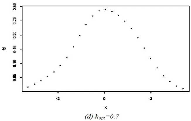
Normal distribution ((N(0,1)) with n = 10 We obtained h oversmoothing bandwidth or hos = 0.53 and CVKL(h) maximum = 0.6. Using the estimating curve with bandwith (h) 0.3 to 0.6, it showed that the optimal bandwith (hopt ) is is the same as CVKL(h) maximum= 0.6, and the estimated curve is shown in Figure 1.

Normal distribution ((N(0,1)) with n = 25 We obtained h oversmoothing bandwidth or hos = 0.65 and CVKL(h) maximum = 0.7. Using the estimating curve with bandwith (h) 0.45 to 0.7, it showed that the optimal bandwith (hopt) is the same as CVKL(h) maximum = 0.7, and the estimated curve is shown in Figure 2.

(3)

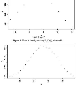
Normal distribution ((N(5,10)) with n = 10 We obtained h oversmoothing bandwidth (hos)

= 4.4 andCVKL(h) maximum = 5. By using the estimating curve with bandwith (h) 3 to 5, it showed that the optimal bandwith (hopt ) is the same as CVKL(h) maximum = 5, and the estimated curve is shown in Figure 3.

Normal distribution ((N(5,10)) with n = 25 We obtained h oversmoothing bandwidth (hos) = 5.3 and CVKL(h) maximum = 6. Using the estimating curve with bandwith (h) 3 to 6, it showed that the optimal bandwith (hopt ) is the same as CVKL(h) maximum = 6, and the estimated curve is shown in Figure 4.

Figure 1. Normal density curve (N(0,1)) with n=10.

(4)

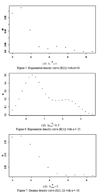
Exponential distribution ((E(1)) with n = 10 We obtained h oversmoothing bandwidth (hos) = 0,97 and CVKL(h) maximum = 1. Using the estimating curve with bandwith (h) 0.5 to 1, it showed that the optimal bandwith (hopt ) is the same as CVKL(h) maximum = 1, and the estimated curve is shown in Figure 5.

Exponential distribution ((E(1)) with n = 25 We obtained h oversmoothing bandwidth (hos) = 0.49 and CVKL(h) maximum = 0.5. Using the estimating curve with bandwith (h) 0.2 to 0.5, it showed that the optimal bandwith (hopt ) is the same as CVKL(h) maximum = 0.5, and the estimated curve is shown in Figure 6.

Gamma distribution (G(1,1)) with n = 10 We obtained h oversmoothing bandwidth (hos) = 1.52 and CVKL(h) maximum = 0.5. Using the estimating curve with bandwith (h) 1 to 2, it showed that the optimal bandwith (hopt ) is the same as CVKL(h) maximum = 2, and the estimated curve is shown in Figure 7.

(5)

Figure 5. Exponential density curve (E(1)) with n=10.

Figure 6. Exponential density curve (E(1)) with n = 25.

(6)

Table 1. Kolmogorov-Smirnov Goodness of Fit Test Distribution

N(0,1) N(5,10) Exponential (1) Gamma (1,1)

Sample size

Dn D0.05 Dn D0.05 Dn D0.05 Dn D0.05

n=10 0.1443ns 0.369 0.1081ns 0.369 0.3920* 0.369 0.4438* 0.369 n=25 0.0879ns 0.283 0.0776ns 0.283 0.2843* 0.283 0.2772* 0.283 Note: ns= nonsignificant at α=0.05

*=significant at α=0.05

Kolmogorov-Smirnov goodness of Fit test The result of Kolmogorov-Smirnov Goodness of Fit Test can be seen in Table 1. We reject hipotesis nul when Dn > D0.05.

By comparing the figures obtained by Kernel Method with Kolmogorof Smirnov test, we can say that both methods gave the same preformance. Figure 1, Figure 2, Figure 3, and Figure 4 showed that the data were normally distributed which were the same as Kolmogorof Smirnov’s (Table 1). The same result were given by Figure 5 and Figure 6 (data from exponential distribution) as well as Figure 7 and Figure 8 (data from Gamma distribution) when comparing with Kolmogorof Smirnov’s (Table 1).

The result is also the same as the result by Ahmad & Mugdadi (2003) which showed that kernel method gave the same performance with the result of Locke & Spurrier (1976) when simulated from distribution different than normal such as from the Chi-Square, the Cauchy and the Beta Distributions.

CONCLUSION

The simulation study illustrates that kernel method is useful for testing normality for n=10 and n=25. This study also reveals that severe

departure from normality can be detected easily using kernel method. By comparing the results from Kernel Method and Kolmogorov Smirnov test, we conclude that the two test gave the same performance

REFERENCES

Ahmad IA & Mugdadi AR. 2003. Testing Normality using Nonparametric Kernel Methods. Jurnal of Nonparametrics Statistics. 15(3): 273-288.

Fan YQ. 1994. Testing Goodness of Fit Tests of a Parametric Density Function by Kernel Method. Econometric Theory. 10: 316-356.

Kvam PH & Vidakovic B. 2007. Nonparametric Statistics with Apllications to Science and Engineering. John Wiley and Sons, New Jersey.

Montgomery DC. 2005. Design and Analysis of Experiment. John Wiley and Sons, New Jersey.

Silverman BW. 1986. Density Estimation for Statistics and Data Analysis. Chapman and Hall Ltd, New York.

Shapiro SS & Wilk MB. 1965. An Analysis of Variance Test for Normality. Biometrika.

52: 591-611