THIS PAGE IS BLANK

THIS PAGE IS

Published by New Age International (P) Ltd., Publishers All rights reserved.

No part of this ebook may be reproduced in any form, by photostat, microfilm, xerography, or any other means, or incorporated into any information retrieval system, electronic or mechanical, without the written permission of the publisher.All inquiries should be emailed torights@newagepublishers.com

ISBN (10) : 81-224-2321-3

ISBN (13) : 978-81-224-2321-1

Price :

£

9.99

PUBLISHING FOR ONE WORLD

NEW AGE INTERNATIONAL (P) LIMITED, PUBLISHERS

DEDICATIONS

I would like to thank my wife Soma, son Anik and

my sister Sujata for giving me a constant support

THIS PAGE IS

PREFACE

A long time ago, about 20–25 years ago, when we used to work on materials with small particles even in the range 4–5 nm, particularly in a magnetic or electronic material, we were not aware that we were actually dealing with nano materials. These materials showed very interesting magnetic or electronic properties, which are the main properties of great concern in the field of modern nano materials or nano composites.

Recently, during the last ten years or so, there has been a surge of scientific activities on the nano materials, or even on commercial products in the marketplace, that are called nano products. Any material containing particles with size ranging from 1 to 100 nm is called nano material, and in this particle size range, these materials show peculiar properties, which can-not be adequately explained with our present-day knowledge. So, the surge on the research activities and the consequent enthusiasm are on the rise by the day.

In the world of materials, like ceramics, glasses, polymers and metals, there has been a considerable activity in finding and devising newer materials. All these new materials in question have extraordinary properties for the specific applications, and most of these materials have been fabricated by newer techniques of preparation. Moreover, they have been mostly characterized by some novel techniques in order to have an edge on the interpretation of the experimental data to be able to elucidate the observed interesting properties.

For example, for oxide and non-oxide ceramics and many metal-composites in powder metallurgy, the sintering of the material is of utmost importance in making hi-tech materials for high performance applications, e.g. in space, aeronautics and in automobiles as ceramic

engine parts. The sintering of these materials to a high density, almost near to the theoretical density, has been possible by using the ‘preparation techniques’, which allow the creation of nano sized particles. Our knowledge on solid state physics and chemistry tells us that these are the materials, or rather the ‘preparation techniques’ to make them, that are fundamentally important to achieve our goal of creating high strength and high performance materials of to-day’s necessity.

Some of these techniques of preparation and characterization of nano materials are elucidated in this book. The subject of ‘nano’ is quite a nascent field and consequently the literature on this emerging subject is not so extensive. Hence, such an attempt, even at the cost of restricting ourselves to a fewer techniques of materials preparation and characterization, is worth in the context of dissemination of knowledge, since this knowledge could be also useful for other nano materials for many other applications.

This book is concerned with the technique of attrition milling for the preparation of nano particles like two important ceramic materials for hi-tech applications, e.g. silicon carbide

The small sized nano particles of magnetite embedded in a glass-ceramic matrix showing interesting magnetic properties would also be highlighted. This is done together with some novel techniques, like Mossbauer Spectroscopy for super-paramagnetic behaviour of nano-sized magnetite and Small Angle Neutron Scattering (SANS) for the determination of nucleation and crystallization behaviour of such nano particles in the chapter 5. The electronic and optical properties of nano particles, which are created within a glassy matrix, would also be elaborated in the chapters 6 and 7, with some mention of the latest developments in these interesting fields of research.

The recent subject like nano-optics, nano-magnetics and nano-electronics, and some such newer materials in the horizon, are also briefly included in this book in the chapter - 8 in order to highlight many important issues involved in the preparation and application of these useful materials.

There is a slight inclination to the theoretical front for most of the subjects, including the mechanical part, discussed in this book. This cannot be avoided by considering the immen-sity of the problem. The whole attempt in this book is devoted to the interests of the materials scientists and technologists working in diverse fields of nano materials. If it raises some form of interest and encouragement to the newer brand of engineers and scientists, then the pur-pose of the book will be well served.

A. K. Bandyopadhyay

ACKNOWLEDGEMENTS

First of all, I would like to thank Professor D. Chakravorty, Ex-Director, Centre of Materials Science, I.I.T. Kanpur, and Ex-Director of Indian Association for the Cultivation of Science, Kolkata, for introducing me to the field of nano materials many years ago.

I would like to thank Professor J. Zarzycki, Ex-Director of Saint Gobain Research, Paris, and Ex-Director, CNRS Glass Lab at Montpellier (France) for giving me a lot of insights on sol-gel materials for preparing nano particles. Of course, I would like to thank Professor J. Phalippou of CNRS Glass Lab at Montpellier, for his help to make me understand the subject of sol-gel processing.

I would like to thank both Dr. J. Chappert and Dr. P. Auric of Dept. of Fundamental Research, Centre of Nuclear Studies at Grenoble (France), for inducting me to the world of magnetic materials and Mossbauer spectroscopy.

I would also like to thank Dr. A. F. Wright of Institut Laue Langevin at Grenoble (France) for introducing me to the subject of Small Angle Neutron Scattering for the study of nano particles.

I would also like to thank M. S. Datta for doing experiments painstakingly on attrition milling and sintering of silicon carbides creating a possibility to prepare a large amount of nano particle-sized materials for many applications like ceramic engines, and many more hi-tech applications for the future.

I would like to thank some of my colleagues in my college, who have shown a lot of interest on nano materials and doing some useful work, and to many staff members, particularly to Mr. S. M. Hossain, to help me prepare the manuscript.

Finally, I would like to give special thanks to Dr. P. C. Ray, Dept. of Mathematics, Govt. College of Engineering and Leather Technology, Kolkata, for his constant help on many scientific issues involving nano physics and continuous encouragements, and special thanks are also due to Dr. V. Gopalan of Materials Science Deptt., Penn. State University (USA), for giving me a lot of insights on Photonics based on ferroelectric materials, and whose work in this field has been a great inspiration to me.

Thanks are also due to Mr. T. K. Chatterjee (RM) and Mr. S. Banerjee (ME) of New Age International, Kolkata, for their constant follow-up to make this work completed.

Author

THIS PAGE IS

CONTENTS

Preface ... (vii)

Acknowledgements ... (ix)

1. General Indroduction ... 1

Preamble ... 1

1.1. Introduction ... 1

1.1.1. What is Nano Technology ? ... 2 1.1.2. Why Nano Technology ? ... 2 1.1.3. Scope of Applications ... 2 1.2. Basics of Quantum Mechanics ... 2 1.2.1. Differential Equations of Wave Mechanics ... 3 1.2.2. Background of Quantum Mechanics ... 6 1.2.3. Origin of the Problem : Quantization of Energy ... 7 1.2.4. Development of New Quantum Theory ... 8 1.2.5. Quantum Mechanical Way : The Wave Equations ... 10 1.2.6. The Wave Function ... 16 1.3. The Harmonic Oscillator ... 19 1.3.1. The Vibrating Object ... 19 1.3.2. Quantum Mechanical Oscillator ... 20 1.4. Magnetic Phenomena ... 23

Preamble ... 23

1.4.1. Fundamentals of Magnetism ... 24 1.4.2. Antisymmetrization ... 25 1.4.3. Concept of Singlet and Triplet States ... 27 1.4.4. Diamagnetism and Paramagnetism ... 28 1.5. Band Structure in Solids ... 31

Preamble ... 31

1.5.1. The Bloch Function ... 31 1.5.2. The Bloch Theorem ... 32 1.5.3. Band Structure in 3-Dimensions ... 35 1.6. Mössbauer and ESR Spectroscopy ... 38 1.6.1. Mössbauer Spectroscopy ... 38

Preamble ... 38

1.6.1.1. The Isomer Shift ... 40 1.6.1.2. The Quadrupole Splitting ... 41 1.6.1.3. The Hyperfine Splitting ... 42 1.6.1.4. Interpretation of the Mössbauer Data ... 42

1.6.1.5. Collective Magnetic Excitation ... 44 1.6.1.6. Spin Canting ... 45 1.6.2. ESR Spectroscopy ... 47

Preamble ... 47

1.6.2.1. The Theory of ESR ... 48 1.6.2.2. ESR Spectra of Iron containing Materials ... 49 1.7. Optical Phenomena ... 50

Preamble ... 50

1.7.1. Electrodynamics and Light ... 50 1.7.2. Transition Dipole Bracket ... 51 1.7.3. Transition Probabilities for Absorption ... 52 1.7.4. The Stimulated Emission ... 55 1.7.5. The Spontaneous Emission ... 56 1.7.6. The Optical Transition ... 58 1.8. Bonding in Solids ... 59

Preamble ... 59

1.8.1. Quantum Mechanical Covalency ... 59

1.9. Anisotropy ... 63

Preamble ... 63

1.9.1. Anisotropy in a Single Crystal ... 63

References ... 65

2. Silicon Carbide ... 67

Preamble ... 67

2.1. Applications of Silicon Carbides ... 67 2.1.1. Important Properties ... 67 2.1.2. Ceramic Engine ... 68 2.1.3. Other Engineering Applications ... 68

2.2. Introduction ... 69

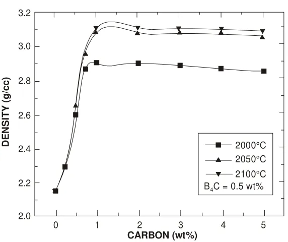
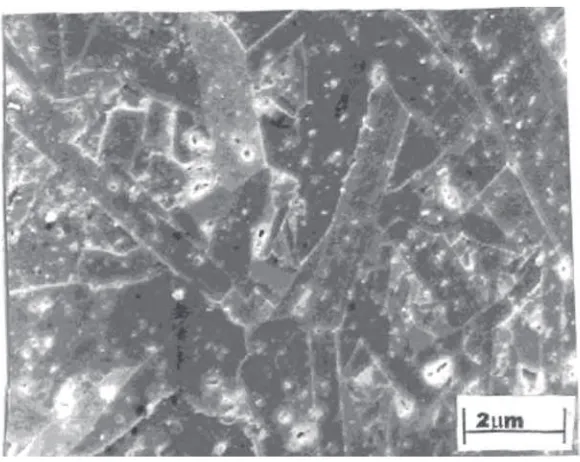
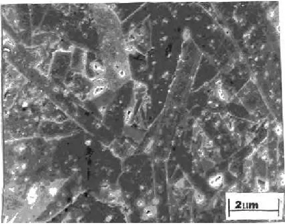
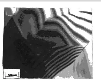
2.4. Sintering of SiC ... 82 2.4.1. Role of Dopants ... 83 2.4.2. Role of Carbon ... 85 2.4.3. Role of Sintering Atmosphere ... 86 2.5. X-ray Diffraction Data ... 86 2.5.1. X-ray Data Analysis ... 87 2.5.2. The Dislocation Mechanism ... 90 2.5.2.1. Dislocation Behaviour ... 90 2.6. Electron Microscopy ... 92 2.6.1. Scanning Electron Microscope ... 92 2.6.2. Sample Preparation for Microstructural Study ... 92 2.6.3. Transmission Electron Microscope ... 92 2.6.4. Sample Preparation for TEM Study ... 93 2.7. Sintering of Nano Particles ... 94 2.7.1. Preparation of Materials ... 94 2.7.2. Sintering of Nano Particles of SiC ... 94 2.7.3. Analysis of the Sintering Data ... 94 2.7.3.1. Role of Aluminum Nitride ... 94 2.7.3.2. Role of Boron Carbide ... 96 2.7.3.3. Effect of Carbon ... 98 2.7.3.4. Effect of Atmosphere ... 108

References ... 113

3. Nano Particles of Alumina and Zirconia ... 117

Preamble ... 117

3.1. Introduction ... 118

3.2. Other Methods for Nano Materials ... 118 3.2.1. Novel Techniques for Synthesis of Nano Particles ... 119 3.3. Nano Material Preparation ... 121 3.3.1. Attrition Milling ... 121 3.3.2. Nano Particles of Alumina ... 121 3.4. Microwave Sintering of Nano Particles ... 125 3.4.1. Microwave Sintering Route ... 126 3.4.2. Sample Preparation from Nano Particles ... 128 3.4.3. Sintering Procedures of Nano Particles ... 128 3.4.4. Sintering Data of Nano Particles of Alumina ... 129 3.5. Characterization ... 129 3.5.1. Electron Microscopy ... 129 3.5.2. Sample Preparation for TEM and SEM Study ... 130

3.6. Wear Materials and Nano Composites ... 131 3.6.1. Nano-Composite Ceramic Materials ... 133 3.6.2. Nano Composite Alumina Ceramics ... 133 3.7. Nano Particles of Zirconia ... 135 3.7.1. Applications of Zirconia ... 135 3.7.2. Synthesis of Nano Particles of Zirconia ... 136 3.7.2.1. Sol-Enulsion-Gel Technique ... 137 3.7.2.2. The Sol-Gel Technique ... 138 3.7.3. Phase Trasnsformation in Nano Particles of Zirconia ... 140 3.7.4. Characteristics of Nano Particles of Zirconia ... 141 3.7.5. Sintering of Nano Particles of Zirconia ... 143

References ... 144

4. Mechanical Properties ... 148

Preamble ... 148

4.1. Theoretical Aspects ... 148 4.1.1. Data Analysis of Theoretical Strength ... 151 4.2. Strength of Nano Crystalline SiC ... 152

Preamble ... 152

4.2.1. The Basic Concepts ... 152 4.2.2. Weibull Theory ... 154 4.2.3. Stress Intensity Factor ... 155 4.3. Preparation for Strength Measurements ... 156 4.3.1. Nano Powder Preparation and Characteristics ... 156 4.3.2. Strength Measurement ... 156 4.3.2.1. Flexural Strength ... 156 4.3.2.2. Fracture Toughness ... 157 4.4. Mechanical Properties ... 157 4.4.1. Comparison of Mechanical Data of α- and β-SiC ... 158 4.4.2. Flexural Strength of α-SiC ... 158 4.4.3. Microstructure ... 162

References ... 167

5. Magnetic Properties ... 169

Preamble ... 169

5.1. Introduction ... 169

5.1.4. The Spinels ... 171 5.1.5. Losses due to Eddy Currents in Magnetic Materials ... 173 5.1.6. Structural Ordering of Ferrites ... 173 5.1.7. The Mechanism of Spontaneous Magnetization of Ferrites ... 174 5.1.8. Magnetization of Ferrites and Hysteresis ... 175 5.2. Super-Paramagnetism ... 177 5.3. Material Preparation ... 180 5.3.1. Nano Particles and X-ray Data ... 181 5.4. Magnetization of Nano Particles of Magnetite ... 181 5.4.1. Variation of Temperature and Magnetic Field ... 183 5.4.2. Magnetic Characteristics of Blank Glass ... 185 5.4.3. Magnetic Characteristics of the 700 and 900 Samples ... 186 5.4.4. Lattice Expansion in Ferrites with Nano Particles ... 190 5.5. Mössbauer Data of Nano Particles of Magnetite ... 192 5.5.1. Hyperfine Field in Nano Particles ... 195 5.5.2. Spin Canting in Nano Particles of Magnetite ... 199 5.6. ESR Spectroscopy ... 202 5.7. Small Angle Neutron Scattering ... 206

Preamble ... 206

5.7.1. Theoretical Considerations ... 207 5.7.2. Nucleation and Crystallization Behaviour ... 207 5.7.3. Small Angle Neutron Scattering ... 212 5.7.4. Interpretation of the SANS Data ... 214 5.7.5. Preparations for the SANS Study ... 215 5.7.6. SANS Data for Nano Particles ... 216 5.7.6.1. Validity of James’ Assumptions ... 217 5.7.6.2. Nucleation Maximum and Guinier Radius of Nano Particles ... 221 5.7.6.3. Ostwald Ripening for Nano Particles and the Growth ... 222 5.7.7. Redissolution Process for Nano Particles ... 223

References ... 227

6. Electrical Properties ... 229

6.1. Switching Glasses with Nano Particles ... 229

Preamble ... 229

6.1.1. Introduction ... 229 6.1.2. Preparation of Glasses with Nano Particles ... 229 6.1.3. Electrical Data of Nano Particles of Bismuth and Selenium ... 231 6.1.3.1. Electrical Conduction in Bismuth Glasses ... 231 6.1.3.2. Electrical Conduction in Selenium Glasses ... 234 6.1.3.3. Tunneling Conduction in Nano Particles ... 237

6.2. Electronic Conduction with Nano Particles ... 242 6.2.1. Introduction ... 242 6.2.2. Preparation of Nano Particles and Conductivity Measurements ... 243 6.2.3. DC Conduction Data of Nano Particles ... 244 6.2.3.1. Correlation between Electronic Conduction ... 245

and Magnetic Data

6.2.4. AC Conduction Data of Nano Particles ... 246 6.2.5. The Verwey Transition of Nano Particles ... 248 6.2.6. Electrical Conductivity of Other Nano Particles ... 250 6.2.7. Impurity States in Electronic Conduction ... 251

References ... 252

7. Optical Properties ... 254

Preamble ... 254

7.1. Introduction ... 254

7.2. Optical Properties ... 255 7.2.1. Some Definitions ... 255 7.2.2. The Refractive Index and Dispersion ... 255 7.2.3. The Non-Linear Refractive Index ... 255 7.2.4. The Absorption Coefficient ... 256 7.2.5. The Reflection ... 256 7.3. Special Properties ... 257 7.3.1. Accidental Anisotropy-Birefringence-Elasto-Optic Effect ... 257 7.3.2. Electro-Optic and Acousto-Optic Effects ... 258 7.3.2.1. The Electro-Optic Effect ... 258 7.3.2.2. The Acousto-Optic Effect ... 259 7.4. The Coloured Glasses ... 260 7.4.1. Absorption in Glasses ... 260 7.4.2. The Colour Centres : Photochromy ... 261 7.4.3. The Colour due to the Dispersed Particles ... 262 7.4.3.1. The Gold Ruby Glass ... 262 7.4.3.2. The Silver and Copper Rubies ... 262 7.4.4. The Luminescent Glasses ... 263 7.4.4.1. The Laser Glasses ... 264 7.4.4.2. Some Examples of Nano Particles ... 266

References ... 267

8. Other Methods and Other Nano Materials ... 269

Preamble ... 269

8.1.1.1. Precursor Alkoxides ... 270 8.1.1.2. Chemical Reactions in Solution ... 271 8.1.1.3. The Process Details ... 272 8.1.1.4. Behaviour of Some Gels ... 273 8.1.2. Electro Deposition ... 275 8.1.2.1. Electro-Deposition of Inorganic Materials ... 276 8.1.2.2. Nano-Phase Deposition Methodology ... 277 8.1.2.3. Electro-Deposition of Nano Composites ... 278 8.1.3. Plasma -Enhanced Chemical Vapour Deposition ... 279 8.1.4. Gas Phase Condensation of Nano Particles ... 280 8.1.4.1. Gas-Phase Condensation Methods ... 280 8.1.5. Sputtering of Nano Crystalline Powders ... 281 8.2. Important Nano Materials ... 282 8.2.1. Nano-Optics ... 282

Preamble ... 282

8.2.1.1. Structure and Function ... 283 8.2.1.2. Preparation of Nano-Optics ... 284 8.2.1.3. Integration Modes ... 285 8.2.1.4. Applications of Nano-Optics ... 286 8.2.1.5. Photonic Band Gap ... 286 8.2.1.6. Optical Chips > Semiconductor to MEMS ... 287 8.2.1.7. Subwavelength Optical Elements (SOEs) ... 288 8.2.1.8. Novel Properties of Nano Vanadium Dioxide ... 290 8.2.2. Nano-Magnetics ... 291 8.2.2.1. Magnetic Semiconductors ... 291 8.2.2.2. Spin Electronics ... 292 8.2.3. Nano - Electronics ... 294

Preamble ... 294

8.2.3.1. The Semiconductors ... 294 8.2.3.2. The Semiconductor Structures ... 295 8.2.3.3. The Quantum Wells ... 295 8.2.3.4. The Quantum Wires ... 295 8.2.3.5. The Quantum Dots ... 296 8.2.3.6. Quantum Computers ... 296 8.3. Other Important Nano Materials ... 296 8.3.1. Microelectronics for High Density Integrated Circuits ... 296 8.3.2. Si/SiGe Heterostructures for Nano-Electronic Devices ... 298 8.3.3. Piezoresistance of Nano-Crystalline Porous Silicon ... 298 8.3.4. QMPS Layer with Nano Voids ... 299 8.3.5. MEMS based Gas Sensor ... 299

References ... 301

THIS PAGE IS

Chapter 1

Chapter 1

Chapter 1

Chapter 1

Chapter 1

General Intr

General Intr

General Intr

General Intr

General Introduction

oduction

oduction

oduction

oduction

PREAMBLE

In 1959, the great physicist of our time Professor Richard Feynman gave the first illuminating talk on nano technology, which was entitles as : There’s Plenty of Room at the Bottom. He

con-sciously explored the possibility of “direct manipulation” of the individual atoms to be effective as a more powerful form of ‘synthetic chemistry’.

Feynman talked about a number of interesting ramifications of a ‘general ability’ to manipulate matter on an atomic scale. He was particularly interested in the possibility of denser computer circuitry and microscopes that could see things much smaller than is possible with ‘scanning electron micro-scope’. The IBM research scientists created today’s ‘atomic force microscope’ and ‘scannin tunneling microscope’, and there are other important examples.

Feynman proposed that it could be possible to develop a ‘general ability’ to manipulate things on an atomic scale with a ‘top → down’ approach. He advocated using ordinary machine shop tools to develop and operate a set of one-fourth-scale machine shop tools, and then further down to one-six-teenth-scale machine tools, including miniaturized hands to operate them. We can continue with this

particular trend of down-scalng until the tools are able to directly manipulate atoms, which will require redesign of the tools periodically, as different forces and effects come into play. Thus, the effect of gravity will decrease, and the effects of surface tension and Van der Waals attraction will be enhanced. He concluded his talk with challenges to build a tiny motor and to write the information from a book page on a surface 1/25,000 smaller in linear scale.

Although Feynman’s talk did not explain the full concept of nano technology, it was K. E. Drexler who envisioned self-replicating ‘nanobots’, i.e., self-replicating robots at the molecular scale, in En-gines of Creation:The Coming Era of Nano Technology in 1986, which was a seminal ‘molecular

nano technology’ book.

That brings us to the end of the brief history on how the concept of nano technology emerged. 1.1. INTRODUCTION

In the usual and standard language, when we talk about ‘materials science’ and ‘materials technol-ogy’, we normally mean ceramics or crystalline materials, glasses or non-crystalline materials, polymers or heavy chain molecular materials and metals or cohesively-bonded materials. All these materials have a wide variety of applications in the diverse fields towards the service for the betterment of human life.

The world of materials is rapidly progressing with new and trendiest technologies, and obviously novel applications. Nano technology is among these modern and sophisticated technologies → which is

creating waves in the modern times. Actually, nano technology includes the concept of physics and chemistry of materials. It beckons a new field coming to the limelight. So, nano technology is an inter-esting but emerging field of study, which is under constant evolution offering a very wide scope of research activity.

1.1.1. What is Nano Technology ?

Nano-technology is an advanced technology, which deals with the synthesis of nano-particles, processing of the nano materials and their applications. Normally, if the particle sizes are in the 1-100 nm ranges, they are generally called nano-particles or materials. In order to give an idea on this size

range, let us look at some dimensions : 1 nm = 10 Å = 10–9 meter and 1 µm (i.e., 1 micron) = 10–4 cm =

1000 nm. For oxide materials, the diameter of one oxygen ion is about 1.4 Å. So, seven oxygen ions will

make about 10 Å or 1nm, i.e., the ‘lower’ side of the nano range. On the higher side, about 700 oxygen

ions in a spatial dimension will make the so-called ‘limit’ of the nano range of materials.

1.1.2. Why Nano Technology ?

In the materials world, particularly in ceramics, the trend is always to prepare finer powder for the ultimate processing and better sintering to achieve dense materials with dense fine-grained micro-structure of the particulates with better and useful properties for various applications. The fineness can reach up to a molecular level (1 nm – 100 nm), by special processing techniques. More is the fineness,

more is the surface area, which increases the ‘reactivity’ of the material. So, the densification or consoli-dation occurs very well at lower temperature than that of conventional ceramic systems, which is finally ‘cost-effective’ and also improves the properties of materials like abrasion resistance, corrosion resist-ance, mechanical properties, electrical properties, optical properties, magnetic properties, and a host of other properties for various useful applications in diverse fields.

1.1.3. Scope of Applications

The deviations from the bulk phase diagram may be exploited to form certain compositions of alloys that are otherwise unstable in the bulk form. In addition, the thermal stability of interfacial regions is typically less than that of the bulk material : thus the nano-phase materials are often sintered or undergo phase transformation at temperatures below those of the bulk material. This is a characteristic which has numerous applications to material processing.

By improving material properties, we are able to find the applications as varied as semiconductor electronics, sensors, special polymers, magnetics, advanced ceramics, and membranes. We need to im-prove our current understanding of particle size control and methodologies for several classes of nano-phase materials and address the issues of their characterization. We should also explore the fields in which there are foreseeable application of nano-phase materials to long standing materials problems, since these ‘issues’ have to be tackled by us.

As said earlier, there is a scope of wider applications in different fields such as : (a) Electronics

in terms of Thin Films, Electronic Devices like MOSFET, JFET and in Electrical Ceramics, (b) Bionics,

(c) Photonics, (d) Bio-Ceramics, (e) Bio-Technology, (f) Medical Instrumentation, etc.

1.2. BASICS OF QUANTUM MECHANICS

atoms themselves, then how we can aspire to know more about the behaviour of the “nano particles”, which are either embedded within a particular matrix or just remain as a mixture in a ‘particulate assem-bly’.

In order to talk about quantum mechanics, we must clarify different aspects of mechanics— which is a pillar in science since the era of ‘Newtonian Mechanics’. Actually, there are four realms of mechnics, which will put quantum mechanics in proper perspectives. The following diagram simply illustrates this point :

Speed ↑ ↑ ↑ ↑ ↑

QUANTUM FIELD THEORY RELATIVISTIC MECHANICS

(Pauli, Dirac, Schwinger, (Einstein)

Feynman, et al.)

QUANTUM MECHANICS CLASSICAL MECHANICS

(Planck, Bohr, Schrodinger, (Newton)

de Broglie, Heisenberg, et al)

Distance→→→→→

Some people say that the subject of quantum mechanics is all about ‘waves’ and that's why sometimes we call it ‘wave mechanics’ in common parlance, yet many textbooks on this subject do not explicitly clarify how the ‘waves’ are created through the mathematical route. When this part is made clear, it has been observed that many readers find quantum mechanics quite interesting. Hence, a simple attempt is made here towards this objective.

1.2.1 Differential Equations of Wave Mechanics

There are so many problems in wave mechanics, which can be described as the ‘solutions’ of a differential equation of the following type :

2 2 d y

dx + f(x) y = 0 (1.1)

The readers studying this subject must thoroughly understand this equation. Here, f(x) is a

func-tion of the independent variable x. With this equation, we can plot y vs. x, when the values of y and 2

2 d y

dx are provided for an arbitrary value of x.

We can also make an equivalent statement : Two independent solutions of y₁ and y₂ exist and

that (Ay₁ + By₂) is the ‘general solution’; this is also possible to be shown graphically.

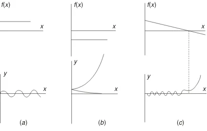
The simplest case of equation (1.1) is that where f(x) is constant. Two cases are possible for this

1. If f(x) is a positive constant, i.e.f(x) = k2, we can write the solution as: y = A cos kx + B sin kx

or, y = a cos (kx + ε)

where, A, B, a and ε are all arbitrary constants. This particular solution is clearly shown in Fig. 1.1(a).

2. If f(x) is constant, but negative, i.e., by setting f(x) = – γ2, we get the solutions as e–γx and eγx,

with the general solution as :

y = A e–γx + B eγx

These solutions are depicted in Fig. 1.1(b).

In the general case, where f(x) is not a constant, it is easy to show that if f(x) is positive →y is an

oscillating function. If f(x) is negative, y is of exponential form.

f x

( )

f x

( )

f x

( )

( )

a

( )

b

( )

c

y

x

y

y

x

x

x

x

x

Figure 1.1 : Solutions of the differential equations y′′ + f(x)y = 0. (a) for f(x) = k2,

(b) for f(x) = – γ2, (c) for an arbitrary form of f(x) that changes sign.

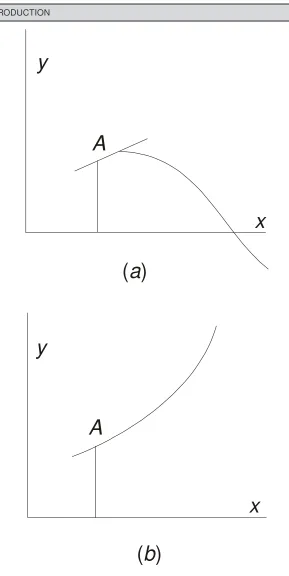
This is due to the fact that if f(x) is positive, both y and 2

2 d y

( )

a

y

A

x

y

x

A

( )

b

On the other hand, if f(x) is negative, both y and 2

2 d y

dx are of the same sign, and the slope at any

point will increase giving an exponentially increasing curve, as shown in Fig. 1.2(b). The general form

of the solution y for a function f(x) which changes sign is as shown in Fig. 1.1(c). When f(x) becomes

negative, y goes over to the ‘exponential’ form. Generally speaking, there will always be one solution

which decreases exponentially, but the general solution will increase. When we consider that the solu-tion consists of an exponential decrease, this determines the phase of oscillasolu-tions in the range of x for

which the oscillations occur

A useful method exists for determining approximate solutions of the differential equation (1.1), known as Wentzel-Kramers-Brillouin (WKB) method, which is written as :

y = αeiβ (1.2)

Here, a and b are both functions of x and α represents the amplitude of the oscillations, β the

phase. The approximate solution of equation (1.2) is written as :

y = Const. f–1/4 exp

Immediately, it follows that the ‘amplitude’ of the oscillations increases, as f becomes smaller

and the wavelength increases (as shown in Fig. 1.1c). So that sums up the basics of waves through a

simple mathematical route, which should clarify the point mentioned above.

1.2.2. Background of Quantum Mechanics

First of all, it could be stated that a knowledge of quantum mechanics is indispensable to under-stand many areas of physical sciences. Quantum mechanics is a branch of science, which deals with ‘atomic’ and ‘molecular’ properties and behaviour on a microscopic scale, i.e., useful to understand the

behaviour of the “nano” particles in the microscopic level. Some salient points can be mentioned as : # It is known that while ‘thermodynamics’ may be concerned with the heat capacity of a gaseous sample → quantum mechanics is concerned with the specific changes in ‘rotational energy states’ of the molecules.

# While ‘chemical kinetics’ may deal with the ‘rate of change’ of one substance to another →

quantum mechanics is concerned with the changes in the vibrational states and structure of the reactant molecules as they get transformed.

# Quantum mechanics is also concerned with the ‘spins’ of atomic nuclei and ‘population of excited states’ of atoms.

# Spectroscopy is based on changes of various quantized energy levels. Thus quantum mechan-ics seem to merge with many other areas of modern science from nuclear physmechan-ics to organic chemistry to semiconductor electronics.

# The modern applications of quantum mechanics have their roots in the development of physics around the turn of the 20th century. Some of the classic experiments date back to 100 years, which provides a solid physical basis for interpretation of quantum mechanics.

1.2.3 Origin of the Problem : Quantization of Energy

So, a little bit of history needs to be told. Before 1900, with proper statistical considerations, the physicists assumed that the laws governing the ‘macroworld’ were valid in the ‘microworld’ → this posed problems in terms of inadequate ‘theory of black-body radiation’ due to Wien’s and Rayleigh-Jeans’ radiation laws.

So, the quantum theory was developed, which had its origin in the lapses of ‘Classical Mechan-ics’, i.e. mechanics, electromagnetism, thermodynamics and optics, to explain experimentally observed

energy (E) vs. wavelength or frequency (v) curves, i.e., distribution, in the ‘continuous spectrum’ of

black-body radiation. Actually, we need to explain the colour of light emitted by an object when heated to a certain temperature. Here, the extraordinary efforts made by Planck needs to be little bit elaborated on how the concept of ‘quantization’ came into existence.

A correct theory of black-body radiation was developed by Max Planck (1857–1947) in 1900, by assuming that the absorption and emission of radiation still arose from some sort of oscillators, which requires that the radiation be ‘quantized’. The fundamental assumption of Planck was that only certain frequencies were possible/permissible for the oscillators instead of the whole range of frequencies, which are normally predicted by classical mechanics. These frequencies were presumed to be some multiple of a fundamental frequency of the oscillators, ν.

Furthermore, Planck assumed that the energy needed to be absorbed to make the oscillator move from one allowed frequency to the next higher one, and that the energy was emitted at the frequency lowered by ν.

Planck also assumed that the change in energy is proportional to the fundamental frequency, ν. By introducing a constant of proportionality, h, i.e., E = hν (h = Planck’s Constant = 6.63 × 10–27 erg sec

= 6.63 × 10–34 _{Joule sec). This famous equation predicted the observed relationship between the}

fre-quency of radiation emitted by a blackbody and the intensity.

In 1905, Albert Einstein (1879–1955) further developed the ‘concept’ of energy quantization by assuming that : this phenomenon was a property of the radiation itself and this process applied to both absorption and emission of radiation. By using the above quantization concept, Einstein developed a correct theory of the ‘photoelectric’ effect.

In 1913, Neils Bohr (1885-1962) combining classical physics and quantization concept postu-lated theory for the observed spectrum of hydrogen atom as follows :

A. The electron in the hydrogen atom moves around the nucleus, i.e. proton, in certain circular

orbits (i.e., stationary states) without radiating energy.

B. The allowed ‘stationary states’ are such that L = m V r = n h (where, L = angular momentum

of the electron, r = radius of the orbit, m = mass of the electron, D =

2

h

π, V = velocity of the electron

with n = principal quantum number).

C. When the electron makes a transition from a state of energy E₁ to E₂ (E₁ > E₂),

electromag-netic radiation (i.e., photon) is emitted from the hydrogen atom. The frequency of this emission process

is given by : ν = (E1 E )2 h −

Bohr’s theory was applied to other atoms with some success in a generalized form by Wilson and Sommerfeld. By about 1924, it was clear that all we needed is a ‘new theory’ to interpret the basic properties of atoms and molecules in a proper manner [1-4]

1.2.4 Development of New Quantum Theory

In 1925, Heisenberg (1901-) developed a system of mechanics where the knowledge of classical concepts of mechanics was revised. The essence of his theory is : Heisenberg assumed that the atomic theory should talk about the ‘observable’ quantities’ rather than the shapes of electronic orbits (i.e.,

Bohr’s theory), which was later developed into matrix mechanics by matrix algebra. Then came the theory of wave mechanics, which was inspired by De Broglie's (1892-) wave theory of matter :

λ = h

p (p = momentum of a particle and λ = wavelength).

Almost parallel to the advancement of matrix mechanics, in 1926 Schrodinger (1887-1961) in-troduced an ‘equation of motion’ based on ‘partial differential equation’ for matter waves, which proved that wave mechanics was mathematically equivalent to matrix mechanics, although its physical meaning was not very clear at first.

But, Why it is so ?

Schrodinger first considered the ‘de Broglie wave’ as a physical entity, i.e., the particle, electron,

is actually a wave. But this explanation has some difficulty, since a wave may be partially reflected and partially transmitted at a ‘boundary’ → but an electron can not be split into two component parts, one for transmission and the other for reflection.

This difficulty was removed by the statistical interpretation of de Brogli wave by Max Born (1882-1970), which is now widely accepted → known as ‘Born Interpretation’. The entire subject was very rapidly developed into a cohesive system of mechanics → called Quantum Mechanics. Since it deals with the waves, we may sometimes call it wave mechanics.

Incidentally, it may be mentioned that the famous German Mathematecian David Hilbert sug-gested to Heisenberg to try the route of ‘partial differential equations’. If Heisenberg listened to Hilbert, then the famous ‘partial differential wave equation’ would be to his credit, but Schrodinger got the Nobel Prize for this most important discovery of the past century in 1933 with Paul Dirac. So, this is the short story of quantum mechanics.

How Schrodinger Advanced His Ideas ?

For the ‘Wave Equation for Particles’, Schrodinger assumed a ‘Wave Packet’ and used Hamiltonian’s ‘Principle of Least Action’. During the development of wave mechanics, it was known to Schrodinger that :

A.Hamilton had established an analogy between the Newtonian Mechanics of a particle and

geometrical or ray optics called Hamiltonian Mechanics, and

B.Equations of wave optics reduced to those of geometrical optics, if the wavelength in the

former is equal to zero.

In order to make a complete description of the ‘motion of the particle’ by the ‘motion of a wave’, we must do the following:

(A) To find a suitable ‘wave representation’ of a single particle, and

(B) To establish the ‘kinematical equivalence’ of a ray and a particle trajectory

A localized wave whose amplitude is zero everywhere, except in a small region, is called the

‘wave packet’, which will satisfy the condition (A), but we have to also satisfy the condition (B).

To Prove the ‘Kinematic Equivalence’ →→→→→ How to Start ?

A monochromatic ‘plane wave’ in one dimension can be represented by :

ϕk(x, t) = ϕ(k) exp[i(kx – ωt)] (1.3)

where, k is the x-component of the propagation vector, denoted by k or | k | = 2π

λ , and ω = ω(k) = 2πν.

It has to be noted that a superposition of a group of plane waves of nearly the same wavelength and frequency that interfere destructively everywhere except in a small region gives rise to a ‘wave packet’. In the one-dimensional case, such a ‘wave packet’ can be represented by ‘Fourier Analysis’, by taking an ‘wave packet’ centered at k which extends to ± Δk so that the ‘Fourier Integral’ can be used between k – Δk/2 and k + Δk/2 as :

the ‘oscillating exponential function’ for different values of k would result on an average in a flat

pat-tern, i.e., a destructive interference.

Let us assume that the form of ψ(0, 0) is:

In order to get a ‘maximum’, we require that :

By neglecting the 2nd _{derivative of ω and the higher order terms in the above expansion,}

ulti-mately we find that the equation (1.7) becomes :

x Now, it is clear how we establish the ‘kinematical equivalence’ of a ‘ray’ and a ‘particle’ trajec-tory, i.e., the condition (B) as explained above, by requiring that the ‘group velocity’ of the ‘wave

packet’ equals the velocity of the particle → which means that :

Vg = Vp (1.10)

and, the momentum is written as :

p = 2m[E – V] = H λ ,

the group velocity of the wave can be written as:

Vg = Now, we have finally established the fact that it is reasonable to consider → describing the motion of a particle by the use of a ‘localised wave’, i.e., wave packet → if we require that E = Constant

× ν. Surprisingly, this is exactly the ‘Planck’s Quantization of Energy Condition’, where H = h (i.e. the

Planck’s Constant), as described earlier.

1.2.5 Quantum Mechanical Way: The Wave Equations

The Postulate 1 →→→→→ For any possible ‘state of a system’, there is a function ψψψψψ, of the coordinates of the parts of the system and time that completely describe the ‘system’.

For a single particle described by the Cartesian coordinates, we can write it as :

ψ = ψ(x, y, z, t) (1.14)

For two particles, the coordinates of each particle must be specified so that :

ψ = ψ(x₁, y₁, z₁, x₂, y₂, z₂, t) (1.15)

For a general system, we can use generalized coordinates q_i , and it is written as :

ψ = ψ(q_i, t) (1.16)

Since the model is that of a wave, the function is called a ‘wave function’. The state of the system which is described by this function is called the ‘quantum state’.

The meaning of this wave function is that ψ2 _{is proportional to the probability. Since ψ may be}

complex, we are interested in ψψ*, where ψ* is the complex conjugate of ψ. The complex conjugate is the same function with i replaced by – i, where i = −1 .

For example →→→→→ If we square the function (x + ib) we obtain : (x + ib) (x + ib) = x2 + 2ib + i2b2

= x2 + 2ib – b2 and the resulting function is still complex. Now, if we multiply (x + ib) by its complex

conjugate (x – ib), we obtain : (x + ib) (x – ib) = x2 – i2b2 = x2 + b2, which is real. Hence, for the

calculation of probability, it is always done by multiplying a function with its complex conjugate. The quantity ψψ* dV is proportional to the probability of finding the particle of the system in the

volume element, dV = dx dy dz. We require that the total probability be unity so that the particle must

be somewhere, i.e., it can be expressed as:

Vψψ*

∫

dV = 1 (1.17)

If this condition is met, then ψ is normalized. In addition, ψ must be ‘Finite’, ‘Single Valued’ and ‘Continuous’. These conditions describe a “well behaved” wave function. The reasons for these require-ments are as follows:

1. Finite. A probability of unity denotes a ‘sure thing’. A probability of zero means that a

par-ticular event can not happen. Hence, the probability varies from zero to unity. If ψ were infi-nite, the probability could be greater than unity.

2. Single valued. In a given area of space, there is only one probability of finding a particle. For

example, there is a single probability of finding an electron at some specified distance from the nucleus in a hydrogen atom. There can not be two different probabilities of finding the electron at some given distance.

3. Continuous. If there is a certain probability of finding an electron at a given distance from the

nucleus in a hydrogen atom, there will be a slightly different probability if the distance is changed slightly. The probability function does not have ‘discontinuities’ so the wave func-tion must be continuous.

If two functions ψ1 and ψ2 have the following property :

1* 2dV ψ ψ

or,

∫

ψ ψ1 2* Vd = 0 (1.18)

They are said to be orthogonal. Whether the integral vanishes or not may depend on the ‘limits of integration’, and hence we always speak of the “orthogonality” within a certain interval.

Therefore, the 'limits of integration’ must be clear. In the above case, the integration is carried out over the possible range of coordinates used in dV. If the coordinates are x, y and z, the limits are from –∞ to

+ ∞ for each variable. If the coordinates are r, θ and φ, the limits of integration are 0 to ∞, 0 to π, and

0 to 2π, respectively.

Postulate 2. For every ‘dynamical variable’ (classical observable), there is a corresponding “operator”.

This postulate provides the ‘connection’ between the quantities which are classical observables and the quantum mechanical techniques for doing things.

But what are the dynamic variables ?

These are such quantities as energy, momentum, angular momentum and position coordinates. The operators are symbols which indicate that some mathematical operations have to be per-formed. Such symbols include ( )2_, d

dx and ∫. The coordinates are the same in operator and classical

forms, e.g., the coordinate x is simply used in operator form as x. Some operators can be combined,

e.g., since the kinetic energy is 2

The operators that are important in quantum mechanics have two important characteristics : 1. First, the operators are linear, which means that :

α(φ1 + φ2) = αφ1 + αφ2 (1.19)

where α is the operator and φ1 and φ2 are the ‘functions’ being operated on. Also, if C is a constant, we

get :

α(Cφ) = C (α φ) (1.20) The linear character of the operator is related to the superposition of 'states' and waves reinforc-ing each other in the process.

2. Secondly, the operators that we encounter in quantum mechanics are Hermitian. If we con-sider two functions φ1 and φ2, the operator α is Hermitian if we have the following relation :

1* 2dV

φ αφ

∫

=

∫

φ α φ2 * 1*dV (1.21)

This requirement is necessary to ensure that the calculated quantities are real. We will come across these types of behaviour in the operators that we use in quantum mechanics.

The Eigenvalues

Postulate 3. The permissible values that a dynamical variable may have are those given by

αφ αφαφ

The postulate can be stated in terms of an equation as :

α φ = a φ (1.22)

operator wave constant wave function (eigenvalue) function

If we are performing a particular operation on the ‘wave function’, which yields the ‘original function’ multiplied by a ‘constant’, then φ is an ‘eigenfunction’ of the operator α. This can be illus-trated by letting the value of φ = e2x and taking the operator as d

dx. Then, by operating on this function

with the operator we get :

d dx

φ

= 2 e2x = constant . e2x (1.23)

Therefore, e2x is an ‘eigenfunction’ of the operator α with an ‘eigenvalue’ of 2. For example,

If we let φ = e2x and the operator be ( )2, we get : (e2x)2 = e4x, which is not a constant times the

which is a constant (nD) times the original (eigen)function. Hence, the ‘eigenvalue’ is _nD.

The Expectation Value

For a given system, there may be various possible values of a ‘parameter’ we wish to calculate. Since most properties (such as the ‘distance’ from the nucleus to an electron) may vary, we desire to determine an average or ‘expectation’ value. By using the operator equation αφ = aφ

where φ is some function, we multiply both sides of this equation by φ* :

φ* α φ = φ* aφ (1.26)

However, it has to be noted that φ*aφ is not necessarily the same as φaφ*. In order to obtain the sum of the probability over all space, we write this in the form of the integral equation as :

Vφ α φ* dV

∫

=

Vφ*aφdV

∫

(1.27)

But ‘a’ is a constant and is not affected by the order of operations. By removing it from the

integral and solving for ‘a’ yields :

It has to be remembered that since α is an operator, φ*αφ is not necessarily the same as αφ*φ, so that the order of φ*α φ must be preserved and α cannot be removed from the integral.

Now, if φ is normalized, then by definition

∫

φ α φ* dV = 1, and we get :

a = < a > =

∫

φ α φ* dV (1.29)

where, a and < a > are the usual ways of expressing the average or expectation value. If the wave

function is known, then theoretically an expectation or average value can be calculated for a given parameter by using its operator.

A Concrete Example →→→→→ The Hydrogen Atom

Let us consider the following simple example, which illustrates the ‘application’ of these ideas. Let us suppose that we want to calculate the ‘radius’ of the hydrogen atom in the 1s state. The

normalized wave function is written as :

ψ1s =

where a₀ is the Bohr radius. This equation becomes :

< r > =

∫

ψ*_1s (operator) ψ_1sdV (1.31)

Here the operator is just r, since the position coordinates have the same form in operator and

classical forms. In polar coordinates, the volume element dV = r2 sin θdrdθdφ. Hence, the problem

becomes integration in three different coordinates with different limits as :

< r > = 2 While this may look rather complicated, it simplifies greatly, since the operator r becomes a

multiplier and the function r can be multiplied. Then the result is written as :

< r > = 2

By using the technique from the calculus, which allows us to separate multiple integrals as :

∫f(x) g(y) dx dy = ∫f(x) dx∫g(y) dy (1.34)

we can write equation (1.33) as :

< r > =

It can be easily verified that :

2

0 0

π π

and the exponential integral is a commonly occurring one in quantum mechanics. It can be easily

evalu-so that we can write the ‘expectation value’ as :

< r > = ₃

Thus, finally, we can get the ‘expectation value’ for the hydrogen 1s state as :

< r >_1s = 1.5 a₀ (a₀ = 0.529 Å) (1.40)

With a probability curve of the electron in 1s state as a function of the distance from the nucleus,

this typical value of the ‘expectation value’ is shown in Fig. 1.3, where the meaning of the maximum of

probability of finding an electron at certain distance and its expectation value are quite different.

Distance in units of a

₀

1.2.6 The Wave Function

Postulate 4. The ‘state’ function, ψψψψψ, is given as a solution of : Hψψψψψ = Eψψψψψ, where, H is the operator for total energy, the Hamiltonian Operator.

This postulate provides a starting point for formulating a problem in quantum mechanical terms, because we usually seek to determine a wave function to describe the system being studied. The Hamiltonian function in classical physics is the total energy, K + V, where K is the translational (ki-netic) energy and V is the potential energy. In operator form :

H = K + V (1.41)

Where K is the operator for kinetic energy and V is the operator for potential energy. If we write in the generalized coordinates, q_i , and time, the starting equation becomes :

Hψ(q_i, t) = – h i ⎛ ⎞ ⎜ ⎟

⎝ ⎠ ∂ψ(qi, t)/∂t (1.42)

The kinetic energy can be written in terms of the momentum as :

K =

Now, we can write it in three dimensions as :

K =

By putting this in operator form, we make use of the momentum operators as :

K = 1

However, we can write the square of each momentum operator as :

2

where ∇2 _{is Laplacian operator or simply Laplacian. The general form of the potential energy can be}

written as :

V = V (q_i, t) (1.48)

So that the operator equation becomes :

This is the famous Schrodinger time-dependent equation or, Schrodinger second equation. In many problems, the classical observables have values that do not change with time, or at least their average values do not change with time. Therefore, in most cases, it would be advantageous to simplify the problem by the removal of the dependence on the 'time'.

How to do it ?

The well known ‘separation of variable technique’ can now be applied to see if the time depend-ence can be separated from the ‘joint function’. First of all, it is assumed that ψ(q_i, t) is the product of

two functions : one a function which contains only the q_i and another which contains only the ‘time’ (t).

Then, we can easily write it as :

Ψ(q_i, t) = ψ(q_i)τ(t) (1.50)

It has to be noted that Ψ is used to denote the complete ‘state’ function and the lower case ψ is used to represent the ‘state’ function with the time dependence removed. The Hamiltonian can now be written in terms of the two functions ψ and τ as :

HΨ(q_i, t) = Hψ(q_i)τ(t) (1.51)

Therefore, the equation (1.49) can be written as :

Hψ(q_i) τ(t) = –

‘time’ (t), so each can be considered as a constant with respect to changes in the values of the other

variable. Both sides can be set equal to some new parameter, X, so that :

1

From the first of these equations, we get :

and from the second one, we get :

The differential equation involving the ‘time’ can be solved readily to give :

τ(t) = e−( / ) Xi D t _(1.58)

By substituting this result into equation (1.50), we find that the total ‘state’ function, Ψ, is :

Ψ(q_i, t) = ψ(q_i) e−( / ) Xi D t (1.59)

Therefore, the equation (1.52) can be written as :

( / ) Xi t

e− D can be dropped from both sides of equation (1.61), which results in :

Hψ(q_i) = Xψ(q_i) (1.62)

which clearly shows that the time dependence has been separated.

Here, neither the Hamiltonian operator nor the wave function is time dependent. It is this form of the equation that could be used to solve many problems. Hence, the time-independent wave function, ψ, will be normally indicated when we write Hψ = Eψ .

For the hydrogen atom, V = –

2 e

r , which remains unchanged in the operator form. Hence, we

can write it as :

which gives rise to the following equation as :

Hψ = Eψ = –

This is the Schrodinger wave equation for the hydrogen atom. Several relatively simple models are capable of being treated by the methods of quantum mechanics. In order to treat these models, we use the above four ‘postulates’ in a relatively straightforward manner. For any of these models, we always begin with :

Hψ = Eψ (1.66)

The quantum mechanical models need to be presented, because they can be applied to several systems which are of considerable interest. For example :

(a) The ‘rigid rotor’ and ‘harmonic oscillator’ models are useful as models in rotational and

vibrational spectroscopy, and obviously for understanding the thermal properties of materials.

(b) The ‘barrier penetration phenomenon’ has application as a model for nuclear decay and

transition state theory (not discussed here).

(c) The particle in a box model has some utility in treating electrons in metals or conjugated

molecules (also not discussed here due to limited applicability).

Out of the above utilities or applications of quantum mechanics, only (a) or Harmonic Oscillator

problem has direct relevance to explain many thermal behaviour of materials, since we need heat to produce a wide range of materials including the “nano materials”.

1.3 THE HARMONIC OSCILLATOR

1.3.1 The Vibrating Object

The vibrations in molecular systems constitute one of the most important properties, which pro-vide the basis for studying molecular structure by various spectroscopic methods (I. R./FTIR, Raman Spectroscopy). Let us start with a vibrating object→→→→→ For an object attached to a spring, Hook’s law

describes the system in terms of the force (F) on the object and the displacement (x) from the

equilib-rium position as:

F = – kx

where k = Spring Constant or Force Constant (Newton. mt or Dynes/cm)

The negative sign means that the resting force or spring tension is in the direction opposite to the displacement. The work or energy needed to cause this displacement (i.e. Potential Energy) is expressed

by the “Force Law”, which is integrated over the interval, 0 to x, that the spring is stretched :

.

If the mass (m) is displaced by a distance of x and released, the object vibrates in simple

har-monic motion. The ‘angular frequency’ of this vibration (ω) is given by:

ω = k

m

where the classical or vibrational frequency (ν) is given by:

ν = 1

Mo-tion, F = m . a. The velocity is the 1st derivative of distance with time dx

This is a linear differential equation with constant coefficients, which can be solved by using the formalism presented above. It is thus seen that the problem of the classical vibrating object serves to introduce the terminology and techniques for the quantum mechanical oscillator, which is much more complex than the classical harmonic oscillator [5 – 6].

1.3.2 Quantum Mechanical Harmonic Oscillator

For studying molecular vibrations and the structure, the harmonic oscillator is a very useful model in quantum mechanics. It was shown in the above description that for a vibrating object, the potential energy (V) is given by:

V = 1₂kx2

which can also be written as:

V = 1₂ mx2ω2

The total energy is the sum of the potential energy and kinetic energy. Now, we must start with the Schrodinger equation as :

Hψ = Eψ

Before we write the full form of the Schrodinger equation, we have to find out →

What is the form of the Hamiltonian Operator ?

Before we find the form of this Hamiltonian operator, the kinetic energy (K) must be known, which is written as :

The potential energy is 2π2_ν2_mx2_{, so that the Hamiltonian operator can now be written as :}

Therefore, the Schrodinger wave equation (Hψ = Eψ) becomes :

By simplifying this equation by multiplying by – 2m and dividing by D2 gives :

2 2 2 2 2

This is the usual form of Schrodinger equation. In this equation, the potential varies as x2, and

since it is a non-linear function, this is much more complex than the classical harmonic oscillator or the particle in the one-dimensional box.

A close look of the above wave equation shows that the “solution” must be a function such that its second derivative contains both the original function and a factor of x2. For very large x, we could

assume that a function like exp(– βx2) satisfies the requirement as : ψ = c[exp(– bx2)]

where, b (= β/2) and c are constants.

The other solution is :

ψ = c[exp(+ bx2)]

which is not a viable solution, since this solution becomes infinity as x → ± ∞, which is in direct

violation of one of the ‘Born conditions’.

In order to check the first solution, we start by taking the required derivatives as :

d

Now, working with the second term of the equation (1.67), we notice that :

– 2 2

It should be noted that both the equations (1.68) and (1.69) contain terms in x2 and terms that do

By canceling the common factors from both sides, we get :

equation. By using the value obtained for b, we can write the ‘solution’ as:

ψ = c

In fact, this is the solution for the harmonic oscillator in its lowest energy state.

The “solution” of the harmonic oscillator problem will now be addressed by starting with the wave equation as :

D , then the differential equation becomes :

2

In order to solve this ‘eigenvalue’ problem, it is now necessary to find a set of wave equations (ψ) which satisfies this equation from – ∞ to + ∞. The function must also obey four ‘Born conditions’. In order to solve the above differential equation, a first solution is found in the limit that x becomes

large. Once x→ ∞ solution is found, a “power series” is introduced to make the large x solution valid

for all x. This is normally called the ‘Polynomial Method’, known since 1880. By the change of

vari-ables to z and after following ‘Born condition’, we arrive at the famous Hermite’s equation. Without

going into a lengthy process, the general form of the Hermite polynomials is written as :

The first few Hermite polynomials can be written as :

The wave functions for the ‘harmonic oscillator’ (ψi) have to be expressed as a normalization

constant (Ni) times Hi(z) to be able to ultimately give a set of normalized wave functions as : ψ0 = N0 exp

The above is just an outline of some of the necessary steps in the full solution of the ‘harmonic oscillator’ model using quantum mechanics [5 – 6]

The above description is useful for vibrational spectroscopy for the determination of various ‘vibration states’ between ‘two bonding atoms’ in a molecule of nano-size or higher. This is obviously useful for some thermal properties like thermal expansion containing various phonon branches, specific heat involving optical and acoustic phonon vibrations in both the longitudinal and transverse modes, and finally on the thermal conductivity that involves the motion of both phonons and electrons. How-ever, in order to have a better knowledge on nano materials, there are many useful properties, like magnetic, electronic and optical, which have to be properly understood in the context of quantum me-chanics [7]. These properties are discussed in some detailes in order get a basic idea about these topics in the following subsections.

1.4 MAGNETIC PHENOMENA

Preamble

In classical physics, a classical charge distribution with angular momentum, which is a ‘rotating’ or ‘spinnng’ charge distribution, gives rise to magnetic moment. Similarly, in quantum mechanics, the ‘angular momentum’ is referred to as ‘electron spin’. In the mathematical treatment of hydrogen by Schrodinger, we get only “three” quantum numbers : n, l and m_l. The subscript l on the magnetic

quan-tum number m_l shows that this m_l value is associated with the orbital angular momentum, which gives

rise to s, p, d and f orbitals, but this treatment does not include the intrinsic angular momentum of the

associ-ated with the ‘intrinsic angular momentum’ of the electron, called s. The m_s is actually the projection of

this momentum on the z-axis, and due to this momentum, the electron has a ‘permanent magnetic

di-pole’. This is how we can see the relation between the ‘electron spin’ and the ‘magnetic moment’. Stern and Gerlach made a ‘dramatic demonstration’ of the existence of ‘electron spin’ by heating silver atom, and making the vapour pass through a baffle and then through an inhomogenous magnetic field (defined as the z-axis) onto a glass plate. This showed two distinct spots for the unpaired 5s

elec-tron of silver 1

2

s

⎛ ₌ ⎞

⎜ ⎟

⎝ ⎠ with two possible projections on the z-axis with ms = ±

1

2. Obviously, it was

already known that a magnetic dipole in an inhomogeneous magnetic field experiences a force, which deflects the ‘dipole’ in a direction that depends on the orientation of the dipole relative to the magnetic field.

1.4.1 Fundamentals of Magnetism

The “spin state” of electrons in an atom determine the magnetic property of the atom. Depending on this spin state of the electrons, the atoms may be classified into mainly : Diamagnetic and Paramag-netic.

(a) Diamagnetic atoms (or ions) are those in which there are no uncoupled or uncompensated

electron spins.

(b) Paramagnetic atoms (or ions) are those with uncoupled or unpaired electron spins in the

orbital giving rise a “net magnetic (spin) moment”.

The magnetic moment of an uncoupled electron is given as Bohr magneton, µB. One Bohr

magneton represents the magnetic moment of ‘one uncoupled’ electron. Therefore, for example, the net magnetic moment for the Fe3+ _{atom is 5µ}

B, since it has ‘5 uncoupled’ electrons. Different types of

magnetism are shown below :

Ferromagnetic Anti-ferromagnetic Anti-ferrimagnetic

Although paramagnetic atoms have ‘net magnetic moments’, the overall magnetic moment of crystalline solid may be zero due to the interaction of the atoms in the crystalline lattice. Depending on the ‘nature’ of this interaction, the atoms may be further classified as ‘ferromagnetic’, ‘anti-ferromagnetic’, ‘ferrimagnetic’.

A crystal is called a ferromagnetic, if the participating atoms are ‘paramagnetic’ and their ‘direc-tions’ are aligned in one direction, which can be switched in the 'opposite direction'. Anti-ferromagnetic crystal is the one whose ‘total magnetic moment’ is zero, since the magnetic moment of the atoms aligned in one direction is compensated by other atoms, whose magnetic moments are aligned in the opposite direction.

up and down moments coexist ‘intrinsically’ within the crystal for ferrimagnetic → while they are formed by two distinct regions (called ‘domains’) of the crystal in ferromagnetic materials. Hence, only ‘one direction’ of magnetic moment exists in a domain of ferromagnetic crystals.

In this book, we are dealing with nano materials. In chapter – 5, the magnetic properties of the

nano particles of magnetite (i.e., a ferrite with a spinel structure) that are embedded in a glassy

diamag-netic matrix are discussed in details. These small particles show a phenomenon of ‘super-paramagnet-ism’ and also within the nano domain for a slightly higher particle size, these nano particles show ‘ferrimagnetism’, as per the above description. In the continuation of this section, we would like to give some details on diamagnetism and paramagnetism along with symmetrization and antisymmetrization, which are very important concepts. Moreover, Pauli’s principle on the ‘electron spin’ is discussed with a mathematical treatment in terms of ‘determinants’ so that a theoretical understanding is developed for the readers to appreciate some intricate details of the ‘magnetic properties’, i.e., the ‘spin properties’, of

nano materials. The necessary concept on the ‘magnetic propetries’ of the nano materials can be ob-tained from the theoretical aspects of Mössbauer and ESR spectra, as detailed in the sections – 1.6.1 and 1.6.2.

The concept of antisymmetrization is important in the quantum level, which can have some cosequences on the magnetic properties of solids containing nano particles. So, here is a brief discussion on this subject.

1.4.2 Antisymmetrization

It is known that the ‘total wave function’ of an electron in a solid consists of a ‘spatial function’ and a ‘spin function’, and for a ‘symmetric spatial function’, the spin function is ‘antisymmetric’, and vice versa. The ‘spatial’ part can be symmetric or antisymmetric. The ‘spin’ part can be symmetric or antisymmetric → but the ‘total function’ must be antisymmetric, since the totally symmetric wavefunction are not valid wave functions.

No additional terms in the Hamiltonian can mix symmetric and antisymmetric states. For the states to mix, a non-zero matrix element must exist. The Hamiltonian including any additional terms is symmetric. The product of a symmetric function and an antisymmetric function is always ‘antisymmetric’. In order to calculate the value of a matrix element, an integration is performed over all space →i.e., in

a symmetric region. Since the product is ‘antisymmetric’, the integral will vanish. Therefore, the ‘totally symmetric’ functions and the ‘totally antisymmetric’ functions are two completely independent to each other, which never mix →i.e., they can have no interaction with each other and hence only one of the

two types of states can exist in nature. This point should be clearly understood.

The Question is →→→→→ Which Type of Function Occurs in Nature ?

This question has been answered by experiments. All experimental observations show that the states occurring in nature are totally ‘antisymmetric’. Let us take an example of He atom, whose ground state is triply degenerate (s = 1) spin state, where the electron spins are ‘unpaired’, if the wavefunction

is totally symmetric → whereas for a ‘non-degenerate’ ground state (s = 0), the spin state, where the

electron spins are ‘paired’, if the wavefunction is totally antisymmetric.

Thes = 1 state would be paramagnetic because of the combined magnetic dipole moments of the

two electrons. By contrast, the s = 0 state is diamagnetic. The experiments show that the ground state of