FAST AND ROBUST SEGMENTATION AND CLASSIFICATION FOR CHANGE
DETECTION IN URBAN POINT CLOUDS
X. Roynarda,∗, J-E. Deschauda, F. Goulettea a
MINES ParisTech, PSL Research University, Centre for robotics, 60 Bd St Michel 75006 Paris, France (xavier.roynard, jean-emmanuel.deschaud, francois.goulette)@mines-paristech.fr
Commission III, WG III/4
KEY WORDS:Urban Point Cloud, Mobile Laser Scanning, Segmentation, Classification, 3D-Features
ABSTRACT:
Change detection is an important issue in city monitoring to analyse street furniture, road works, car parking, etc. For example, parking surveys are needed but are currently a laborious task involving sending operators in the streets to identify the changes in car locations. In this paper, we propose a method that performs a fast and robust segmentation and classification of urban point clouds, that can be used for change detection. We apply this method to detect the cars, as a particular object class, in order to perform parking surveys automatically. A recently proposed method already addresses the need for fast segmentation and classification of urban point clouds, using elevation images. The interest to work on images is that processing is much faster, proven and robust. However there may be a loss of information in complex 3D cases: for example when objects are one above the other, typically a car under a tree or a pedestrian under a balcony. In this paper we propose a method that retain the three-dimensional information while preserving fast computation times and improving segmentation and classification accuracy. It is based on fast region-growing using an octree, for the segmentation, and specific descriptors with Random-Forest for the classification. Experiments have been performed on large urban point clouds acquired by Mobile Laser Scanning. They show that the method is as fast as the state of the art, and that it gives more robust results in the complex 3D cases.
1. INTRODUCTION
With the recent availability of massive urban point clouds, we see an interest in automatic segmentation and classification of this data for numerous tasks dealing with city analysis and survey-ing. Such as emergency simulation, accessibility analysis, city modelling, itinerary planning, maintenance, all kind of network management (rails, road ,electricity, telecommunication, water, gas, etc).
Then we need to extract semantic data of the point clouds, what can be summarized in giving a segmentation and a classification of the point clouds in relevant objects. And for the application of change detection, being able to compare different segmented clouds. In the case of parking surveys, we must detect and seg-ment sub-clouds that represent parked cars, then compare them between different passages.
There are already methods (Serna and Marcotegui, 2014) that automatically segment and classify urban point clouds in reas-onable time. But this methods project the point clouds in 2D and lose a lot of information, as cars under trees or pedestrians under balcony.
We propose an automatic algorithm to segment and classify urban point clouds in similar processing time, but keeping 3D informa-tion and then with more robustness.
The point cloud is projected on a 2D-grid for ground extraction by region-growing. Then we project the cloud on a 3D-grid for object segmentation. We calculate 3D descriptors on each seg-mented object. Finally using a Random-Forest model to perform classification.
∗Corresponding author
Our method has enabled us to create a sufficiently large dataset to test the classification algorithm. We test the classification per-formance and the importance of each descriptor used. In addition we measure the computation time for each step of the method to identify bottlenecks.
This paper is organized as follows. Section 2. reviews related work in the state of the art. Section 3. explains our methodology. Section 4. describes the experiments we used to give the results in section 5., and conclude in section 6..
2. RELATED WORK
There are multiple methods of segmentation and classification of urban point clouds, but we can at first distinguish between meth-ods using a 2D information (either by projecting the cloud of an elevation image, or directly using range images) and meth-ods working directly on the 3D information. Also the way the two steps segmentation and classification can combine may dif-fer greatly from one method to another. Indeed, one can start by segmenting objects and classify each object, but one can also classify each point and use this classification to group points into “real” objects.
autonomous vehicles in real-time, indeed they allow for fast re-gistration on pre-processed 2D maps (Kammel et al., 2008, Fer-guson et al., 2008). Markov Random Fields can be used for con-textual classification (Munoz et al., 2009), or for learning seg-mentation (Anguelov et al., 2005).
Direct point classification: Another approach is to first clas-sify each point by studying its neighbourhood, then group them into relevant objects. This raises the problem of choosing the size of the neighbourhood. This problem is addressed in (Demantk´e et al., 2011) by choosing the size that minimizes an entropy com-puted on features extracted from covariance matrix of the neigh-bourhood called dimensionality features. This method proposes to classify each point in a geometric class: line, surface, volume. This dimensionality attributes are used in several methods (Douil-lard et al., 2011). There are also many local 3D descriptors as VFH estimating normal distributions (Rusu et al., 2010) or RSD using the curvature radius(Marton et al., 2010a) that can be used to build global descriptors of objects CVFH (Aldoma et al., 2011) and GRSD (Marton et al., 2010b).
Detection, Segmentation, Classification: The pipeline which seems the most successful is the following (Golovinskiy et al., 2009): a) ground extraction, b) object detection, c) object seg-mentation, d) supervised learning classification. It was improved by (Velizhev et al., 2012) with object centres estimation and Im-plicit Shape Model for classification instead of supervised learn-ing.
3. PROPOSED METHODOLOGY
In a framework inspired by (Golovinskiy et al., 2009), we propose the following workflow:
extract the ground,
segment the remaining 3D point cloud in connected com-ponents (no detection step, that appears to be unnecessary in three dimensions),
compute a feature vector on each segmented object with 3D descriptors,
classify each object.
3.1 Ground Extraction
After testing several methods including RANSAC and Region-Growing on normal distribution, we chose the following method. We project the point cloud on an horizontal grid discretized with a stepδxy, keeping in each pixelPonly the minimal applicate value:zmin(P) = min
p∈Ppz.
First, we find a pixel which has supposedly a lot of his points on the ground. For this purpose, we compute an histogram inzof the whole point cloud and we find the biggest bin, then we find the pixel of the 2D-grid which has the most points in this bin in proportion to all its points.
Then we grow a regionRfrom this seed, adding a neighbour QofP ∈ Rto the region only if|zmin(P)−zmin(Q)|< δz, whereδzis a parameter to be chosen big enough to allow a certain slope of the ground, but small enough to avoid taking cars and buildings.
The last step is to filter the points in the regionR, indeed, in chosen pixels there might be remaining points not belonging to the ground. That’s why we keep only pointsp∈ Pwhich verify
pz< zmin(P) + ∆in each pixel. Where∆is a threshold which must be bigger than twice the noise of the data around plane.
3.2 Object Segmentation
To segment the objects, we extract the connected components of the remaining cloud. As we seek to maintain reasonable com-putation times, we avoid to achieve a Region Growing directly on the point cloud, what is very time-consuming because of the nearest-neighbour search. Instead, we project the point cloud on a 3D-occupancy-grid or an Octree of resolutionδto be chosen large enough to avoid over-segmentation, and small enough to avoid several objects to be segmented together (for example cars parked too close to each other). Finally we realize a Region-Growing on the occupancy-grid, it is much faster as the neigh-bourhoods are known in this structure.
In our experiments, it seems that optimal choice ofδis always between10cmand15cm.
3.3 Object Classification
3.3.1 Features: For each segmented object we compute a vec-tor of features composed of Geometric features mainly inspired by (Serna and Marcotegui, 2014) and of 3 histogram-based des-criptors from the literature, namely CVFH (Aldoma et al., 2011), GRSD (Marton et al., 2010b) and ESF (Wohlkinger and Vincze, 2011). In summary we obtain a feature vector with991variables: 22for geometric features,308for CVFH,21for GRSD and640 for ESF.
Geometric features: This features are mainly inspired by (Serna and Marcotegui, 2014), they give more robustness to histogram-based descriptor which describe only the local geometry of ob-jects.
First of all, we project horizontally the point cloud on its(x, y) variables to compute the convex hull in 2D and covariance mat-rix of the point cloud in variables(x, y). Then we compute the following geometric features:
the number of points,
zmax−zmin, the area of the 3D convex hull, the volume of the 3D convex hull,
a 10-bins histogram inz.
The 2 following descriptors are histogram-based originally used to recognize objects and their 6DOF-pose of known models, but we use it only for the first task. They both need normal computa-tion, what can be very time-consuming.
CVFH (Clustered Viewpoint Feature Histogram): VFH des-criptor (Rusu et al., 2010) is a concatenation of 4 histograms rep-resenting normal angles distribution on the surface of the object. As VFH is sensitive to noise, CVFH is build by adding a Shape Distribution histogram that can differentiate the clouds that have similar normal distributions, but the points are distributed differ-ently.
whereαis the angle between the normals of the points. This feature seems enough discriminative to distinguish plane, sphere, corner, edge and cylinders. But instead of using the radiusr, RSD is the histogram indandαthat can be used to classify each point of the object.
To build a feature vector globally on the object, the point cloud is projected on an octree, and each voxel is classified using RSD. GRSD is build as GFPFH (Rusu et al., 2009) by observing rela-tionships between this locally labelled voxels.
ESF (Ensemble of Shape Functions): ESF descriptor is based on the idea that the distribution of distances between pairs of points randomly chosen in the object appears to be relevant to classify an object (Osada et al., 2001). Other distributions are important as angles, surfaces and volumes. To further improve performance, each pair of points is classified in “in””, “out”” or “mixed”” depending on whether the segment between these points is inside the object, outside or both. A great benefit of this descriptor is that it does not require the computation of normals, and is therefore much faster than the previous two descriptors.
3.3.2 Classifier: In our work, Random-Forest (Breiman, 2001) are chosen because they are one of the most accurate general pur-pose classifier and have multiple advantages compared to SVM for example, with similar results (Mountrakis et al., 2011) or Gaussian Mixture Model (Lalonde et al., 2005), Markov Random Fields (Munoz et al., 2009) and Adaboost (Lodha et al., 2007).
Random-Forest are part of variance reduction methods by bag-ging (bootstrap aggregating). The principle is to train independ-ently a big number of decision tree, each one on a random subset of the training set (typically two third), and using each time only a random subset of features. Then, in testing time to obtain a prediction on the forest, simply test on each tree and count the number of votes for classification (or average for regression).
The greatest advantages of Random-Forest are:
they give an estimation of error of generalization (out-of-bag: OOB) after training, as each tree is trained only on two third of the dataset, the model can be tested on the last third,
for each feature vector they give the probability to be in each class,
they give importance of each feature, measuring the number of times they are used for training, this allows us to achieve feature selection and potentially reduce computation time,
they are poorly sensitive to parameter changes, what makes them very easy to tune.
4. EXPERIMENTS
4.1 Implementation
All algorithms are implemented in C++ with an intensive use of PCL (Rusu and Cousins, 2011) to read and write PLY files, to compute normals and to compute descriptors such as CVFH, GRSD and ESF. The framework run on one thread except the computation of normals which is parallelised with OpenMP.
For classification, computations are less intensive we use thepython
library scikit-learn (Pedregosa et al., 2011), which provides all features of Random-Forest as OOB score and features import-ance.
The experiments are run on a desktop Intel Core i7 4790K with 4 cores clocked at4GHz.Moreover the computer has32GBof RAM, what allows us to run our algorithms on massive point clouds of more than 100 million points.
4.2 Dataset
All point clouds used for our experiments are acquired with the MLS prototype of the center for robotics of Mines Paritech: L3D2 (Goulette et al., 2006) (as seen in Figure 1). It is a Citro¨en Jumper equipped with a GPS (Novatel FlexPak 6), an IMU (Ixsea PHINS in LANDINS mode) and a Velodyne-HDL32 LiDAR mounted in almost horizontal position.
Figure 1: MLS prototype: L3D2
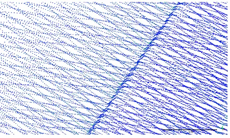
The Dataset is composed of seven pass of650min Paris1 (rue Madame and rue Cassette, 75006 Paris) and seven pass of1.6km in Lille2 (rue du Professeur Perrin and rue Jean Jaur`es, 59170 Croix) at about two hours apart. The clouds have high dens-ity with between 1000 and 2000 points per square meters on the ground, but there are some anisotropic patterns due to the multi-beam LiDAR sensor as seen in Figure 2.
Figure 2: Anisotropic pattern on the ground (color of points is the reflectance)
1
https://www.google.fr/maps/dir/48.8512675,2. 3320095/48.8509089,2.3307348/@48.8496176,2.3311634, 466m/data=!3m1!1e3!4m9!4m8!1m5!3m4!1m2!1d2.3313488! 2d48.8483308!3s0x47e671d0662c1f71:0x3468592da4fea104! 1m0!3e0?hl=en
2
5. RESULTS
5.1 Evaluation: Segmentation
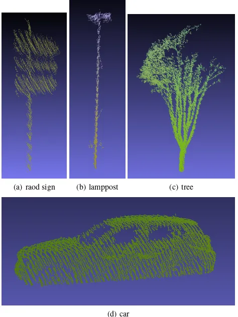
Ground Extraction: The ground extraction step works well on all the dataset, in the sense that the road and the sidewalk is com-pletely extracted. But an inherent consequence of our method is that the lowest points of each object are classified as belonging to the ground (as seen in figure 3(d)).
(a) raod sign (b) lamppost (c) tree
(d) car
Figure 3: Exemple of sub-clouds well segmented after ground extraction
Object Segmentation: There are a lot of artefacts: small sub-clouds that doesn’t represent objects, for example in tree canopy or behind the buildings (as seen in figure 4). We won’t use this artefacts in the Dataset for classification results, but in view of giving a class to each point of the point cloud, we should add a class “artefacts”.
Figure 4: Exemple of ground extraction and object segmentation on a truncated point cloud of Lille (ground in red, and every other object has a different color)
We segment the whole dataset and obtain 20121 objects, most of them being artefacts. Then we classify by hand a few objects
that seem well segmented, to train a first time on classifier which will give us class of other samples when it is confident enough. This allows us to create a dataset quickly. We finally have3906 samples in9classes, but only7of them have enough samples to evaluate classification as seen in Table 1.
Class Number of samples
Paris Lille Total
trees 64 373 437
cycles 142 1 143
buildings 111 404 515
lampposts 16 357 373
pedestrians 10 1 11
poles 508 65 573
trash cans 8 1 9
road signs 114 456 570
cars 719 556 1275
Total 1692 2214 3906
Table 1: Number of samples for each class
5.2 Evaluation: Classification
In Random-Forest the only parameter that can influence classi-fication is the number of trees. Figure 5 shows that OOB error converges when number of trees increases. The choice of256 trees in the Random-Forest is made because more trees would in-crease computation time without real improvement in accuracy, and less trees would decrease accuracy too much.
100
101
102
103
10−2 10−1
Number of trees in the Random-Forest
Error
Out-Of-Bag
10−1
100
101
102
T
raining
time
[s
]
Error Out-Of-Bag Training time
Figure 5: Importance of number of trees in the forest
To evaluate our choices in term of classification we compute 4 indicators that are the precisionP, the recallR, the F1 score and the Matthews Correlation CoefficientM CCas computed in equations 1.
P = T P
T P+F P
R= T P
T P+F N (1)
F1 = 2T P
2T P+F P+F N
M CC =p T P·T N−F P·F N
whereT P, T N, F P andF N are respectively the number of true-positives, true-negatives, false positives and false negatives.
We train the Random Forest Model with 256 trees on the well segmented object in 7 classes that have a sufficient number of samples: trees, cycles, buildings, lampposts, poles, road signs and cars. For training we use90%of the dataset in each class, then we compute precision, recall, F1 and MCC on the remaining 10%, results are shown in table 2.
Class Precision Recall F1 MCC
trees 93.90% 95.84% 94.83% 94.19%
cycles 79.10% 96.00% 86.45% 86.44%
buildings 93.00% 98.69% 95.73% 95.13%
lampposts 90.09% 99.00% 94.28% 93.79%
poles 92.98% 99.69% 96.19% 95.60%
road signs 93.09% 99.40% 96.12% 95.52%
cars 96.97% 99.53% 98.23% 97.37%
Table 2: Mean Precision, Recall, F1 and MCC scores for each class
5.3 Feature importances
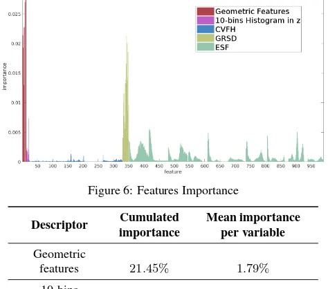
Random-Forest provide an importance for each feature that rep-resent how much it is used to build the model. The importance is shown in figure 6 and table 3 for each descriptor. First of all, it seems that CVFH is almost useless both in cumulative and pro-portionally to number of variables. Although Geometric Features and GRSD have less variables than other descriptors they seem very important. Moreover the descriptor which has the most im-portance cumulatively is ESF, but imim-portance is spread over all its640variables.
Figure 6: Features Importance
Descriptor Cumulated Mean importance importance per variable
Geometric
features 21.45% 1.79%
10-bins
histogram inz 2.01% 0.20%
CVFH 3.93% 0.01%
GRSD 23.09% 1.10%
ESF 49.52% 0.08%
Total 100% 0.10%
Table 3: Cumulated importance of each descriptor and Mean im-portance per variable (given by Randon-Forest).
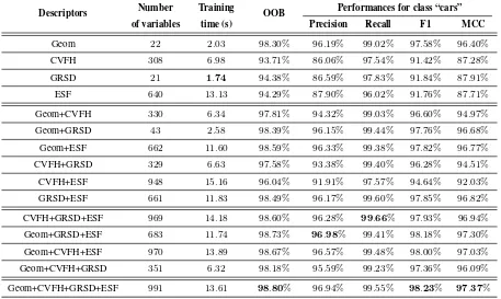
To further investigate the importance of each descriptor we test every possible combination, and draw performance of classifica-tion for class “car” in table 4.
We can conclude that if we want to keep only descriptor which don’t require normal computation: Geometric Features and ESF, we loose only0.21%of OOB score. This is a compromise to be done as the normals are the most time consuming part of the computation of descriptors (as seen in 5.4).
5.4 Computation Time
5.4.1 Segmentation: This corresponds to the time of projec-tion of the point cloud on a 2D-grid and a region growing on this grid for Ground Extraction, then the same thing on a 3D-grid for Object Segmentation. On our dataset, we measure similar times for Ground Extraction and Object Segmentation around25sfor sections of 10 million points. However, the 3D-grid structure has not it been optimized (e.g. using a Octree), we can think that the results could be better.
5.4.2 Descriptors: The time to compute a feature vector highly depends on the number of points of the object, that’s why we give the mean computational time for each descriptor on the 20121 ob-jects segmented in Paris and Lille Dataset.
Two descriptors require the computation of normals on the object, and the operation can be very-time consuming (as shown in table 5) especially for large clouds.
5.4.3 Classification: It seems that the time to predict the class of a feature vector is weakly dependent on the number of vari-ables. Once the Random Forest is trained with 256 trees, predic-tion time per sample is about1.2ms. Thus assuming that feature vectors are computed fast enough, we could predict the class of 833objects each second. Hence the classification is clearly not the bottleneck in our algorithm.
5.5 Comparison with state-of-the-art
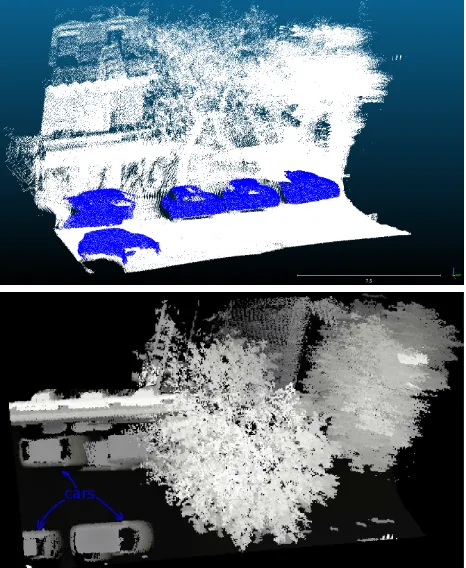
For segmentation, keeping the 3D structure of the point clouds al-lows to segment vehicles under trees as shown in Figure 7. What was not possible with elevation images.
Purely on the classification of cars, we compared with (Serna and Marcotegui, 2014). We obtain a better Recall, but Precision slightly below as seen in Table 6.
6. CONCLUSION
In this work, we proposed an automatic and robust approach to segment and classify massive urban point clouds in reasonable time without using elevation images.
First, the ground is extracted using a Region Growing onzmin kept in an horizontal 2D-grid. Next, the remaining point cloud is segmented in connected components of a 3D-occupancy-grid. Finally, each object is classified using Random-Forest and a fea-ture vector composed of geometric feafea-tures and histogram-based features of the literature.
Descriptors Number Training OOB Performances for class “cars”
of variables time (s) Precision Recall F1 MCC
Geom 22 2.03 98.30% 96.19% 99.02% 97.58% 96.40%
CVFH 308 6.98 93.71% 86.06% 97.54% 91.42% 87.28%
GRSD 21 1.74 94.38% 86.59% 97.83% 91.84% 87.91%
ESF 640 13.13 94.29% 87.90% 96.02% 91.76% 87.71%
Geom+CVFH 330 6.34 97.81% 94.32% 99.03% 96.60% 94.97%
Geom+GRSD 43 2.58 98.39% 96.15% 99.44% 97.76% 96.68%
Geom+ESF 662 11.60 98.59% 96.33% 99.38% 97.82% 96.77%
CVFH+GRSD 329 6.63 97.58% 93.38% 99.40% 96.28% 94.51%
CVFH+ESF 948 15.16 96.04% 91.91% 97.57% 94.64% 92.03%
GRSD+ESF 661 11.83 98.49% 96.17% 99.60% 97.85% 96.82%
CVFH+GRSD+ESF 969 14.18 98.60% 96.28% 99.66% 97.93% 96.94%
Geom+GRSD+ESF 683 11.74 98.73% 96.98% 99.41% 98.18% 97.30%
Geom+CVFH+ESF 970 13.89 98.67% 96.57% 99.48% 98.00% 97.03%
Geom+CVFH+GRSD 351 6.32 98.18% 95.59% 99.23% 97.36% 96.09%
Geom+CVFH+GRSD+ESF 991 13.61 98.80% 96.94% 99.55% 98.23% 97.37%
Table 4: Performances for each combination of descriptor possible (Geom is for Geometric features, for each column the best result is inbold)
Descriptors Computation Time (s) Proportion Mean Time per object (ms)
Geom 17.2 3.22% 0.9
CVFH 240.3 44.92% 11.9
GRSD 64.4 12.04% 3.2
ESF 213.0 39.82% 10.6
Total 534.9 100% 26.6
Normales 964.7 47.9
Table 5: Mean Computational Time of descriptors on20121segmented objects of 7 passes in Lille and Paris
Method Precision Recall F1
(Serna and
Marcotegui, 2014) 100.0% 94.6% 97.2%
ours 96.97% 99.53% 98.23%
Table 6: Classification results for class “car” (inbold the best results)
state of the art. Moreover, we conduct a study of the importance of each descriptor, in order to reduce computation time.
With such classification results, it is possible to achieve change detection on particular classes such as cars. Then between two passages in the same street, we can detect cars that have changed by comparing the corresponding sub-clouds and achieve parking survey. On an other scale of time between acquisitions we can automatically detect the bent poles or road signs.
In our future works, we believe we can improve the accuracy by adding contextual descriptors (such as the elevation of objects above the ground or the number of neighbouring objects) that would avoid classifying as car objects that are in height and re-move segmentation artefacts behind the buildings facades.
REFERENCES
Aldoma, A., Vincze, M., Blodow, N., Gossow, D., Gedikli, S., Rusu, R. B. and Bradski, G., 2011. Cad-model recognition and 6dof pose estimation using 3d cues. In: Computer Vision Work-shops (ICCV WorkWork-shops), 2011 IEEE International Conference on, IEEE, pp. 585–592.
Anguelov, D., Taskarf, B., Chatalbashev, V., Koller, D., Gupta, D., Heitz, G. and Ng, A., 2005. Discriminative learning of markov random fields for segmentation of 3d scan data. In: Com-puter Vision and Pattern Recognition, 2005. CVPR 2005. IEEE Computer Society Conference on, Vol. 2, IEEE, pp. 169–176.
Breiman, L., 2001. Random forests. Machine learning 45(1), pp. 5–32.
Demantk´e, J., Mallet, C., David, N. and Vallet, B., 2011. Di-mensionality based scale selection in 3d lidar point clouds. The International Archives of the Photogrammetry, Remote Sensing and Spatial Information Sciences 38(Part 5), pp. W12.
Figure 7: Example of situation where the method of (Serna and Marcotegui, 2014) does not allow to segment cars located under a tree. Up: 3D point cloud with cars well segmented (in blue), down: max elevation image of the same point cloud where cars located under the tree do not appear.
Ferguson, D., Darms, M., Urmson, C. and Kolski, S., 2008. De-tection, prediction, and avoidance of dynamic obstacles in urban environments. In: Intelligent Vehicles Symposium, 2008 IEEE, IEEE, pp. 1149–1154.
Golovinskiy, A., Kim, V. G. and Funkhouser, T., 2009. Shape-based recognition of 3d point clouds in urban environments. In: Computer Vision, 2009 IEEE 12th International Conference on, IEEE, pp. 2154–2161.
Gorte, B., 2007. Planar feature extraction in terrestrial laser scans using gradient based range image segmentation. In: ISPRS Work-shop on Laser Scanning, pp. 173–177.
Goulette, F., Nashashibi, F., Abuhadrous, I., Ammoun, S. and Laurgeau, C., 2006. An integrated on-board laser range sensing system for on-the-way city and road modelling. The International Archives of the Photogrammetry, Remote Sensing and Spatial In-formation Sciences.
Hoover, A., Jean-Baptiste, G., Jiang, X., Flynn, P. J., Bunke, H., Goldgof, D. B., Bowyer, K., Eggert, D. W., Fitzgibbon, A. and Fisher, R. B., 1996. An experimental comparison of range image segmentation algorithms. Pattern Analysis and Machine Intelli-gence, IEEE Transactions on 18(7), pp. 673–689.
Kammel, S., Ziegler, J., Pitzer, B., Werling, M., Gindele, T., Jag-zent, D., Schr¨oder, J., Thuy, M., Goebl, M., Hundelshausen, F. v. et al., 2008. Team annieway’s autonomous system for the 2007 darpa urban challenge. Journal of Field Robotics 25(9), pp. 615– 639.
Lalonde, J.-F., Unnikrishnan, R., Vandapel, N. and Hebert, M., 2005. Scale selection for classification of point-sampled 3d sur-faces. In: 3-D Digital Imaging and Modeling, 2005. 3DIM 2005. Fifth International Conference on, IEEE, pp. 285–292.
Lodha, S. K., Fitzpatrick, D. M. and Helmbold, D. P., 2007. Aer-ial lidar data classification using adaboost. In: 3-D Digital Ima-ging and Modeling, 2007. 3DIM’07. Sixth International Confer-ence on, IEEE, pp. 435–442.
Marton, Z.-C., Pangercic, D., Blodow, N., Kleinehellefort, J. and Beetz, M., 2010a. General 3d modelling of novel objects from a single view. In: Intelligent Robots and Systems (IROS), 2010 IEEE/RSJ International Conference on, IEEE, pp. 3700–3705.
Marton, Z.-C., Pangercic, D., Rusu, R. B., Holzbach, A. and Beetz, M., 2010b. Hierarchical object geometric categorization and appearance classification for mobile manipulation. In: Hu-manoid Robots (HuHu-manoids), 2010 10th IEEE-RAS International Conference on, IEEE, pp. 365–370.
Mountrakis, G., Im, J. and Ogole, C., 2011. Support vector ma-chines in remote sensing: A review. ISPRS Journal of Photo-grammetry and Remote Sensing 66(3), pp. 247–259.
Munoz, D., Vandapel, N. and Hebert, M., 2009. Onboard con-textual classification of 3-d point clouds with learned high-order markov random fields. In: Robotics and Automation, 2009. ICRA’09. IEEE International Conference on, IEEE.
Osada, R., Funkhouser, T., Chazelle, B. and Dobkin, D., 2001. Matching 3d models with shape distributions. In: Shape Mod-eling and Applications, SMI 2001 International Conference on., IEEE, pp. 154–166.
Pedregosa, F., Varoquaux, G., Gramfort, A., Michel, V., Thirion, B., Grisel, O., Blondel, M., Prettenhofer, P., Weiss, R., Dubourg, V., Vanderplas, J., Passos, A., Cournapeau, D., Brucher, M., Per-rot, M. and Duchesnay, E., 2011. Scikit-learn: Machine learning in Python. Journal of Machine Learning Research 12, pp. 2825– 2830.
Rusu, R. B. and Cousins, S., 2011. 3D is here: Point Cloud Library (PCL). In: IEEE International Conference on Robotics and Automation (ICRA), Shanghai, China.
Rusu, R. B., Bradski, G., Thibaux, R. and Hsu, J., 2010. Fast 3d recognition and pose using the viewpoint feature histogram. In: Intelligent Robots and Systems (IROS), 2010 IEEE/RSJ Interna-tional Conference on, IEEE, pp. 2155–2162.
Rusu, R. B., Holzbach, A., Beetz, M. and Bradski, G., 2009. Detecting and segmenting objects for mobile manipulation. In: Computer Vision Workshops (ICCV Workshops), 2009 IEEE 12th International Conference on, IEEE, pp. 47–54.
Serna, A. and Marcotegui, B., 2014. Detection, segmentation and classification of 3d urban objects using mathematical morpho-logy and supervised learning. ISPRS Journal of Photogrammetry and Remote Sensing 93, pp. 243–255.
Velizhev, A., Shapovalov, R. and Schindler, K., 2012. Implicit shape models for object detection in 3d point clouds. In: Interna-tional Society of Photogrammetry and Remote Sensing Congress, Vol. 2.
Wohlkinger, W. and Vincze, M., 2011. Ensemble of shape func-tions for 3d object classification. In: Robotics and Biomimet-ics (ROBIO), 2011 IEEE International Conference on, IEEE, pp. 2987–2992.