LEICA DMC III CALIBRATION AND GEOMETRIC SENSOR ACCURACY
C. Mueller a, K. Neumann b
Z/I Imaging GmbH, Aalen, Germany –[email protected] Z/I Imaging GmbH, Aalen, Germany –[email protected]
KEY WORDS: Leica DMC III, CMOS, Calibration Method, Geometric Accuracy, Grid Distortion
ABSTRACT:
As an evolution of the successful DMC II digital camera series, Leica Geosystems has introduced the Leica DMC III digital aerial camera using, for the first time in the industry, a large-format CMOS sensor as a panchromatic high-resolution camera head. This paper describes the Leica DMC III calibration and its quality assurance and quality control (QA/QC) procedures. It will explain how calibration was implemented within the production process for the Leica DMC III camera. Based on many years of experience with the DMC and DMC II camera series, it is know that the sensor flatness has a huge influence on the final achievable results. The Leica DMC III panchromatic CMOS sensor with its 100.3mm x 56.9mm size shows remaining errors in a range of 0.1 to 0.2μm for the root mean square and shows maximum values not higher that 1.0μm. The Leica DMC III is calibrated based on a 5cm Ground Sample Distance (GSD) grid pattern flight and evaluated with three different flying heights at 5cm, 8cm and 11cm GSD. The geometric QA/QC has been performed using the calibration field area, as well as using an independent test field. The geometric performance and accuracy is unique and gives ground accuracies far better than the flown GSD.
1. INTRODUCTION
The first single CCD array for the large format digital frame camera, Z/I DMC II, was introduced to the market in 2010. With this introduction, the geometric performance increased by an order of magnitude of the initial performance. With the DMC II development, the geometric calibration moved from an Australis Model base to a Grid-based calibration. A two-step calibration had been performed using a collimator measurement as an initial calibration and enhanced the geometric accuracy by introducing a distortion grid correction.
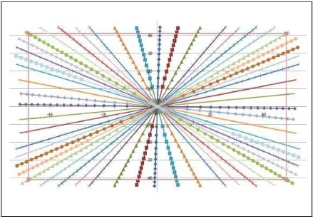
The Z/I DMC II geometric calibration takes place at Carl Zeiss Jena on a certified test stand. More than 800 “light targets”, projected on 28 lines that are distributed diagonally on the focal plane, are automatically measured by finding their light centers with a precision of less than 1/10 of a pixel. The light targets are projected from “infinity” using a collimator (Figure 1).
Figure 1. Light Target Pattern by Collimator SYNTHETIC Light Target Simulation
The grid-based calibration procedure can model aspheric lenses and much more accurately models local distortions. The Leica DMC III uses the same lens system that was employed for the Z/I DMC II 140 and 230 models. It is equipped with a very large single CMOS sensor with a physical size of 26112 x 15000 pixels, with a pixel size of 3.9μm. The Leica DMC III cannot be calibrated using the calibration procedure established for the Z/I DMC II series (using the standard calibration stand at the Zeiss factory), due to calibration stand’s limited positioning accuracy of the camera in front of the collimator. For the pixel size of 3.9μm, the targeted 1/10-of-a-pixel-measuring performance cannot be achieved.
As a solution, a so-called “SYNTHETIC” geometric calibration was established, which is based on a simulated mathematical lens distortion calculation based on the detailed optical design data of the lens. It is equivalent to the DMC II collimator calibration procedure, projecting 800 “light targets” on 28 lines that are distributed diagonally on the focal plane (Figure 1). The large sensor size across flight direction maximizes the utilization of the optical circle. This in turn increases the amount of distortion on the outer edges of the image frame. The challenge of the new calibration concept was to achieve the same or better geometric performance that was obtained with the DMC II camera models.
2. FLIGHT CALIBRATION BLOCK
To perform a DMC III geometric in-field calibration, a well- defined calibration field is required (Figure 2). Some general requirements for the calibration field must first be fulfilled. A square calibration field over the city of Aalen was used, covering this field with a grid pattern of 5 flight lines in the North-South direction and covering the same area with 5 flight lines in the East-West direction. The Ground Sample Distance (GSD) for the calibration purpose is 5cm, and the whole calibration field is well distributed with visible control points. To ensure the calibration procedure, the 2.5x2.5km² calibration The International Archives of the Photogrammetry, Remote Sensing and Spatial Information Sciences, Volume XL-3/W4, 2016
field is covered by 90-95 ground control points (GCPs) with a high horizontal and vertical accuracy. The standard deviation of the available GCPs is 2-3cm in the horizontal direction and 3-4cm in the vertical direction. If some GCPs are covered by objects, there are always many alternative points available. The flight lines are planned with a 75% forward and 75% side overlap to achieve a huge number of multi-ray object points. For the calibration procedure an almost flat terrain over an urban area is preferred to achieve a constant GSD over the block. For final geometric calibration of the multispectral camera sensors, sharp contours are needed within the calibration field. In addition, the area should not include a large number of large trees. Since trees are objects that move with wind, they have a negative impact to the color registration during the calibration procedure. However this paper covers the geometric calibration procedure for the PAN sensor only, since this is relevant for the Leica DMC III geometric performance only.
Figure 2. Leica DMC III calibration flight footprints overlap with Ground Control Point distribution
The calibration procedure is based on highly accurate GNSS/IMU data, therefore it is recommended to have a GNSS ground station within the calibration field to achieve the highest DGNSS accuracy. To achieve the best possible GNSS/IMU accuracies, a couple of requirements for the practical flight performance must to be addressed. About 3-5 minutes before the first exposure is taken, a so-called in-air alignment (figure-8 or S-curve) (Figure 3) needs to be performed to achieve highest IMU data quality. The same procedure needs to be performed 3-5 minutes after the last exposure was taken. The flight lines need to be flown in an alternating procedure (Figure 3) to eliminate systematic influences such as a smaller datum shift, small errors in aircraft GNSS antenna offsets, and to be able to compute the sensor-specific principle point of Auto Collimation (PPAC).
Figure 3. Alternating flight procedure
3. CALIBRATION PROCEDURE
During the geometric calibration for the Leica DMC III camera, the knowledge of the sensor flatness, its tilting against the nadir position with respect to the optical axis and the lens distortion needs to be determined and represents the geometric calibration procedure. The interior flatness of the sensor itself is determined during the production at the factory (Figure 4) and is excluded when exceeding ±30μm.
Figure 4. Manufacturers’ Sensor Flatness measurement
1
2
3
4
5
6 7
8 9
10
The geometric calibration for the Leica DMC III is divided into 4 calibration steps.
1. SYNTHETIC BRONZE
2. BRONZE SILVER 3. SILVER GOLD
4. GOLD PLATINUM
It is an iterative process in which the last step represents the final QC/QA step and provides the final camera accuracy, which serves for validating the targeted sensor accuracy and the calibrated focal length and principle point of auto collimation.
For the calibration steps 1-3 a fully-triangulated Intergraph ISAT project was used that follows the grid calibration guidelines. A grid calibration is used because, in contrast to an Australis model, it is able to represent aspheric lenses, and it can model local distortions more precisely. For steps 1-3, the image standard deviation is relaxed to 8μm (Table 1), and calibration-frame images are used (Figure 5). The full-calibration-frame images are used to get a more precise knowledge of the image distortions at the borders and edge parts of the sensor. The result is a more precisely computed distortion grid for the final image size. For the final image a reduced image size of 25728 x 14592 pixels is used. The mechanical FMC makes this size reduction necessary.
Figure 5. DMC III nominal and absolute image frame size
Calibration Step Image points
Control Points
GNSS StDev
INS StDev StDev X, Y Z X, Y, Z Ω, Φ Κ
[μm] [cm] [cm] [deg]
SYNTHETICBRONZE 8 3 4 4 0.006 0.01
BRONZE SILVER 8 3 4 4 0.006 0.01
SILVER GOLD 8 3 4 4 0.006 0.01
GOLD PLATINUM 3 3 4 4 0.006 0.01
Table 1. a priori AT calibration settings and standard deviations
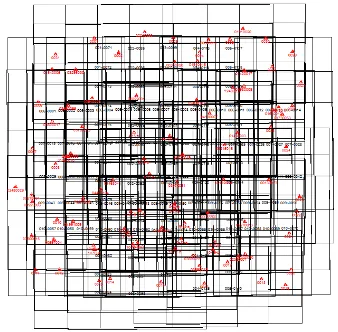
The grid flight pattern provides a very dense image point distribution over the whole block. All image points overlaid to one image (Figure 6) show the consistent image point distribution, which is the base to generate a highly precise grid and to model the image distortions precisely. The calibration block contains 140 exposures (in average there are 275 image points per exposure available) ranging from approximately 140 – 370 image points per image.
Figure 6. All image points overlaid to one image
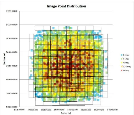
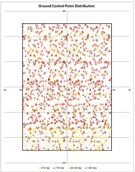
The number of multi-ray image points (Figure 7) and the number of multi-ray GCPs (Figure 8) represent one more indication of the very stable triangulation block and, as a consequence, an indicator for the stability of the post-correction grid and the precision of the distortion model.
Figure 7. Image point distribution over the triangulation block The International Archives of the Photogrammetry, Remote Sensing and Spatial Information Sciences, Volume XL-3/W4, 2016
Figure 8. All ground control points overlaid to one image and color-coded with respect to their numbers of measured rays
During the first calibration step, the ImagePipeMathModel (IPMM), a grid of overlapped 4th -order 2D polynomials (the so-called CGC_SYNTHETIC.ply file) is generated. In addition to this, the ImageStation project should have GNSS/IMU EOs imported including a preliminary misalignment calibration. The misalignments are calculated based on the first run of bundle block adjustment on the available GCPs. This information is used to estimate the sensor focal length and principle point of Auto Collimation. During each calibration step, a clean-up for image point outliers is performed and becomes increasingly more strict (Table 2) from one calibration iteration step to the next, since the remaining distortion becomes smaller and smaller.
Calibration Step Tie/Pass Tie Control Points
σ0 rays σ0 X, Y Z
SYNTHETICBRONZE > 14μm ≤ 2 > 25μm 6cm 9cm
BRONZE SILVER > 8μm ≤ 2 > 14μm 4cm 5cm
SILVER GOLD > 8μm ≤ 2 > 8μm 4cm 5cm
GOLD PLATINUM > 8μm ≤ 2 > 8μm 3cm 4cm Table 2. a posteriori clean-up criteria for AT calibration steps On each calibration step, a post-correction grid file is generated. The number of columns and rows in the grid file accumulates image residuals in the camera frame. It is recommended for DMC III cameras to use roughly 1024x1024 pixel collection cells per quadrant. Two by Two quadrants are used that results in a total cell number of [15000 26112]/1024 = [14.6484 25.5000], which rounds up to 2*[15 26] = [30 52] total number of cells.
For each calibration iteration, a post-calibration tool produces the IPMM file, based on the generated post-correction grid file for the next calibration iteration step (Table 3). It always refined the previous calibration for its remaining non-linear systematic
distortion trend in the focal plane that could not be absorbed by the optimal selection of the focal length and principle point of Auto Collimation, which is only a scale/bias type of correction. The final calibration step, GOLD PLATINUM, is not another step of grid refinement. It is used to scale the GOLD calibration grid calibration from its calibrated to its nominal focal length and principle point of auto collimation.
Calibration Step Input IPMM file
Output IPMM file
SYNTHETIC BRONZE
CGC_SYNTHETIC.ply CGC_BRONZE.ply
BRONZE SILVER CGC_BRONZE.ply CGC_SILVER.ply
SILVER GOLD CGC_SILVER.ply CGC_GOLD.ply
GOLD PLATINUM CGC_GOLD.ply PGC_PLATINUM.ply Table 3. Evolution of the IPMM grid calibration file
4. LEICA DMC III CAMERA GEOMETRY The camera geometry is expressed by the image geometry that means the systematic image errors describing the difference between the real image geometry and the mathematical model of the perspective geometry (Jacobsen, Neumann 2012).
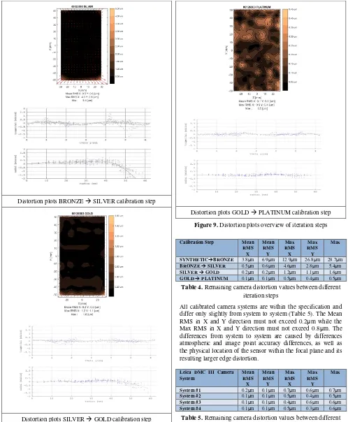
Based on the calibration procedure, the remaining image distortions are getting reduced significantly from one calibration iteration step to the next (Figure 9 and Table 4). The final QA/QC step is performed to estimate the final remaining image distortion. A grid distortion plot, as well as a separated transversal and radial distortion plot, is produced and published within the camera calibration report. Furthermore, a bundle block adjustment analysis is performed, based on a typical photogrammetric block.
Distortion plots SYNTHETIC BRONZE calibration step The International Archives of the Photogrammetry, Remote Sensing and Spatial Information Sciences, Volume XL-3/W4, 2016
Distortion plots BRONZE SILVER calibration step
Distortion plots SILVER GOLD calibration step
Distortion plots GOLD PLATINUM calibration step
Figure 9. Distortion plots overview of iteration steps
Calibration Step Mean
RMS X
Mean RMS Y
Max RMS X
Max RMS Y
Max
SYNTHETICBRONZE 3.8μm 6.9μm 12.9μm 26.8μm 28.7μm
BRONZE SILVER 0.5μm 0.6μm 4.6μm 2.8μm 5.4μm
SILVER GOLD 0.2μm 0.2μm 1.2μm 1.1μm 1.6μm
GOLD PLATINUM 0.1μm 0.1μm 0.5μm 0.4μm 0.5μm
Table 4. Remaining camera distortion values between different iteration steps
All calibrated camera systems are within the specification and differ only slightly from system to system (Table 5). The Mean RMS in X and Y direction must not exceed 0.2μm while the Max RMS in X and Y direction must not exceed 0.8μm. The differences from system to system are caused by differences atmospheric and image point accuracy differences, as well as the physical location of the sensor within the focal plane and its resulting larger edge distortion.
Leica DMC III Camera System
Mean RMS X
Mean RMS Y
Max RMS X
Max RMS Y
Max
System #1 0.2μm 0.1μm 0.7μm 0.6μm 0.7μm
System #2 0.1μm 0.1μm 0.5μm 0.4μm 0.5μm
System #3 0.1μm 0.1μm 0.4μm 0.6μm 0.6μm
System #4 0.1μm 0.1μm 0.5μm 0.3μm 0.6μm
Table 5. Remaining camera distortion values between different camera systems
The averages of the root mean squares of the residuals shown in Table 5 do not exceed 0.2μm and shows the largest values below or equal to 0.7μm. The final PLATINUM calibration shows no obvious systematic trend; almost all systematic effects that were clearly visible within the iteration steps 1 (SYNTHETIC BRONZE) and 2 (BRONZE SILVER) are elimiated. Some systems show slight radial distortion effects at The International Archives of the Photogrammetry, Remote Sensing and Spatial Information Sciences, Volume XL-3/W4, 2016
the image corners and Y-direction edges due to fact that the sensor is coming very close to the brink of the optics.
5. EVALUATION AND TEST DATA SETS 5.1 Block Layouts
The geometric performance of the Leica DMC III was checked with different evaluations and test flights. The main evaluation datasets are taken with a 5cm GSD over the city of Aalen and with a 5cm GSD close to the city of Nördlingen. A second evaluation flight was performed with an 8cm GSD over the city of Aalen and with an 11cm GSD over the Nördlingen area. The 11cm evaluation dataset was taken in a double cross pattern flight instead of a block layout flight. This was mainly used to check the performance of the calibrated nominal focal length. Two more test datasets were taken over a customer airfield with a 7cm and 14cm GSD. The performance of the Leica DMC III was proven using a block layout with and without cross flight lines. The red surrounded ground points were used as control points, while non-surrounded points were used as check points (Figure 10).
GSD 5cm Aalen, end lap 70%, side lap 50% 3 + 2 cross strips
GSD 5cm Noerdlingen, end lap 60%, side lap 40% 4 + 2
cross strips
GSD 8cm Aalen, end lap 60%, side lap 60% 2 + 2 cross strips
GSD 11cm Noerdlingen, end lap 80, 2 + 2 double crossing
strips
GSD 7cm test set, end lap 80%, side lap 60% 3 + 2 cross
strips
GSD 7cm test set, end lap 80%, side lap 60% 3 strips
GSD 14cm test set, end lap 70%, side lap 60% 4 + 2 cross
strips
GSD 14cm test set, end lap 70%, side lap 60% 4 strips
Figure 10. Flight pattern with control and check point configurations for evaluations and test datasets
5.2 Point Accuracy
All evaluation and test datasets display different configurations, different GSDs, and different numbers of control and check points, as well as different end- and side overlaps for all datasets. Therefore, comparisons are not very easy. To make a comparison more meaningful, fully-given RMS and Residual (Figures 11 – 14) values are given in a portion of one pixel. The 5cm GSD dataset with 60/40% overlap is the closest to a typical photogrammetric block. Even the 5cm GSD Aalen block, with 70/50% overlap is a good reference. Nevertheless, independent from the above-mentioned criteria, the geometric performance of the Leica DMC III can be detected.
Figure 11. RMS of check points for different blocks and configurations as described
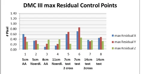
Figure 12. Max Residuals of check points for different blocks and configurations as described
Figure 13. RMS of control points for different blocks and configurations as described
Figure 14. Max Residuals of control points for different blocks and configurations as described
The block adjustments for all evaluation and test datasets show similar results and trends. The average Root Mean Square in horizontal direction of the check points is at 0.41 of a pixel, The average Root Mean Square in vertical direction for the check points is at 0.65 of a pixel. The results are depending on the block configuration, the overlap and the number of check and control points used. In one single evaluation case the maximum horizontal Root Mean Square was 0.66 of a pixel and the maximum vertical Root Mean Square was 0.92 of a pixel. The target is a horizontal RMS of 0.50 of a pixel in horizontal and 0.70 of a pixel in vertical.
6. INFLUENCES OF PERIPHERAL SYSTEMS The in-flight calibration accuracy of a Leica DMC III is not a sensor-and-calibration-procedure-specific task; it is rather influenced by peripheral systems as well. It is without question that all peripheral systems must perform as accurately and precisely as possible to achieve a highly-qualified geometric camera calibration. Two peripheral systems that influence the sensor geometry most significantly are the mechanical Forward Motion Control (FMC) and the stabilization of the sensor during the image release procedure.
6.1 Mechanical FMC and its geometric influence
With the Leica DMC III Pan (CMOS Sensor) a new technique for the forward motion compensation (FMC) is introduced in the DMC family. While for CCD sensor the well-known Time Delayed Integration (TDI) is used. For CMOS this approach is not possible due to different read out strategies. The CMOS sensor must be moved mechanically to correct for the forward motion influence.
For this the Leica DMC III Pan camera head is equipped with a brushless drive; it is a DC-Motor with a gear and an excentric, that moves the sensor carriage.
The Figure 15 is showing the movement and acceleration of the sensor in respect to exposure start. It is shown that the sensor is accelerated shortly before exposure start and moves with a constant speed during shutter opening. Following the sensor movement it will slow down and the sensor moves back to its starting position for the next exposure.
The measurement is done with a very accurate device achieving an accuracy of 50 nm.
Figure 15. FMC Movement in respect to shutter opening and exposure start
For the geometric accuracy it is important that the interior orientation (sensor position) will not change over all exposures. Also the movement of the sensor during exposure should coincide with the real movement over the ground.
To simplify we assume that during the short exposure time period there is no change in flying speed and height over ground, so that the sensor should move linear. Figure 16 is showing the absolute difference from the linearity of one exposure, while Figure 17 and Figure 18 displays the standard deviation from the linearity of one flight project.
Figure 16. Difference to linear movement
Figure 17. FMC standard deviation in μm The International Archives of the Photogrammetry, Remote Sensing and Spatial Information Sciences, Volume XL-3/W4, 2016
Figure 18. FMC standard deviation in number of pixels
At the end the linear movement has only a small influence to the image geometry. More important is to have a constant internal orientation of the sensor. For this a nominal position is defined (here -200μm). Any difference to this nominal position will be corrected automatically during image processing to achieve a positioning accuracy of 1/78 of a pixel. Figure 19 gives an example of a real flight about the IO at exposure start (Red line nominal position)
Figure 19. FMC Start Position
In general the actual positions are influenced by exposure time and mechanical inaccuracies.
The performance above shows that FMC does not have a significant disadvantages compared to TDI regarding image geometry, the opposite is true. Due the possibility of sub-pixel correction a higher performance can be achieved. TDI is able to correct for full pixels only while the FMC has a theoretical standard deviation of 1μm which is ¼ of a pixel. Practical experiences are showing a much better performances, with a standard deviation of ⅛ of a pixel only.
6.2 Sensor stabilization and its geometric influence
Any sensor movement during the exposure release will cause a radiometric image degradation, in the form of blurring.. Those will be greatest at the image corners. For geometric calibration purposes, the radiometric effects are not the most important issues, rather the pixel displacement must be highlighted. This results in a geometric pixel displacement, which influences the final computed sensor distortion model.
Figure 20 shows a unifilar drawing of the 3-dimensional influences of image motions during exposure release. The following equations (1) – (5) were used to calculate and analyse the number of pixel displacements during a calibration flight. The corner point of a Leica DMC III image was taken (the largest pixel displacement effects are visible at this extreme point).
Figure 20. Corner pixel displacement vector
(1)
where = nominal vector from focal point to image corner = altered vector from focal point to image corner X, Y, Z = single components of nominal vector X’, Y’, Z’ = single components of altered vector D = 3 dimensional Rotation matrices
F = focal point f = focal length
(2)
Rotation about fixed axes
where a11…a33 = single coefficients of the 3D Rotation matrices
DΩ = Rotation matrices around X axis DΦ = Rotation matrices around Y axis DΚ = Rotation matrices around Z axis
(3)
where Ω = Rotation angle around X axis Φ = Rotation angle around Y axis Κ = Rotation angle around Z axis
(4)
where = difference between nominal and altered vector dX, dY, dZ = single components of vector
differences
(5)
where dPix = total pixel displacement
Figure 21 shows the angular rate values measured during the Leica DMC III calibration flight for each exposure. The angular rate reflects the portions of the aircraft movements that could not be compensated by the stabilized mount. The maximum angular rate measured during the calibration flight was 0.0384deg/sec and the maximum standard deviation was 0.0108deg/sec. These very small uncompensated aircraft movements cause very small pixel displacements shown in Figure 22.
Figure 21. Max angular rate during exposure release
Figure 22. Max pixel displacement on image corner
The largest pixel displacement was measured with 0.0742 portion of a pixel and the overall standard deviation was computed with 0.0158 portion of a pixel. Thes very small pixel displacement values have no influence on the geometric calibration since the effects are below 1/10 of a pixel. It does, however, need to be taken into account and be analyzed, because there are many stabilized mounts on the market providing a much lower stabilization performance.
CONCLUSION
With the Leica DMC III the overall performance is another step forward compared to any other previous developed large format digital DMC camera type. All analysed blocks taken by the different Leica DMC III sensors are showing systematic image errors in a sub pixel range. The object point accuracies are below one GSD in all 3 directions. It achieves in most cases the 0.70 of a pixel range criterion in vertical direction and 0.50 of a pixel range criterion in horizontal direction.
The analysis of the peripheral systems, like FMC and camera stabilization do not show significant influences to the geometric performance of the Leica DMC III.
The smaller pixel size, the high performant FMC and the high performant camera stabilization provided by the gyro-stabilised sensor mount makes the contribution to perform flights with a very small GSD (down to 3cm). Practical experiences showed very stable and sharp image results even for this challenging ground resolution. This overtakes the operating conditions of most other digital aerial cameras on the market, with respect to geometric accuracy and blurring free image data.
REFERENCES
Albertz/Wiggenhagen, 2009. Guide for Photogrammetry and Remote Sensing, 5th completely revised and extended edition. Wichmann, pp. 43-44.
Collete, F., Gline, S., Losseau, J., Lecharlier, L., 2012. Geometric properties of a mechanical Forward Motion Compensation system controlled by a piezoelectric drive. In:
International Archives of the Photogrammetry, Remote Sensing and Spatial Information Sciences, Volume XXXIX-B5, 2012 XXII ISPRS Congress, 25 August – 01 September 2012, Melbourne, Australia.
Jacobsen, K., Neumann, K., 2012. Property of the large format digital aerial camera DMC II. Commission I, WG I/2.