Learning and process improvement during production ramp-up
Christian Terwiesch
!
,
*
, Roger E. Bohn
"
!Department of Operations and Information Management, The Wharton School, 1319 Steinberg Hall-Dietrich Hall, Philadelphia, PA 19104-6366, USA
"University of California, San Diego, CA, USA
Received 2 June 1999; accepted 18 October 1999
Abstract
Rapid product lifecycles and high development costs pressure manufacturing"rms to cut not only their development times (time-to-market), but also the time to reach full capacity utilization (time-to-volume). The period between completion of development and full capacity utilization is known as production ramp-up. During that time, the new production process is ill understood, which causes low yields and low production rates. This paper analyzes the interactions among capacity utilization, yields, and process improvement (learning). We model learning in the form of deliberate experiments, which reduce capacity in the short run. This creates a trade-o! between experiments and production. High selling prices during ramp-up raise the opportunity cost of experiments, yet early learning is more valuable than later learning. We formalize the resulting intertemporal trade-o!between the short-term opportunity cost of capacity and the long term value of learning as a dynamic program. The paper also examines the tradeo!between production speed and yield/quality, where faster production rates lead to more defects. Finally, we show what happens if managers misunderstand the sources of learning. ( 2001 Elsevier Science B.V. All rights reserved.
Keywords: Yield; Ramp-up; Start-up; Learning curve; Experimentation
1. Introduction
Many high-tech industries are characterized by shrinking product lifecycles and increasingly expensive production equipment and up-front costs. The market window for selling many prod-ucts has shrunk to less than a year in industries such as disk-drives and telecommunications. These forces pressure organizations to cut not only their development times (time-to-market), but also the time it takes to reach full production volume
(time-*Corresponding author. Tel.:#215-898-854.
E-mail address:[email protected] (C. Terwiesch).
to-volume) in order to meet their"nancial goals for the product (time-to-payback).
The period between the end of product develop-ment and full capacity production is known as
production ramp-up. Two con#icting factors are characteristic of this period: low production capacity, and high demand. High demand arises because the product is still `relatively freshaand might even be the"rst of its type. Thus, customers are ready to pay a premium price. Yet output is low due to low production rates and low yields. The production process is still poorly understood and, inevitably, much of what is made does not work properly the "rst time. Machines break down, setups are slow, special operations are needed to
correct product and process oversights, and other factors impede output. Over time, with learning about the production process and equipment, yields and capacity utilization go up (although in many industries they never reach 100%). Due to the con#icts between low e!ective capacity and high demand, the company "nds itself pressured from two sides, an e!ect referred to as the ` nut-crackera[1].
A recent example of the importance of ramp-up can be found in AMD's e!orts to compete with Intel in the microprocessor market. AMD had sev-eral generations of product that were slow to ramp, leading to limited market acceptance and"nancial di$culties for AMD. More recently, Intel experi-enced problems ramping up the yield of its 0.18 micron version of the Pentium. Industry observers speculate that an e!ective ramp-up of AMD's K7 processor will allow AMD to compete in the high end segment of the PC market (Electronic Buyers'
News, June 21, 1999).
In this article, we analyze the interactions among capacity utilization, yields, and yield improvement (learning) during ramp-up. Traditional learning-curve models implicitly assume that manufacturing performance increases with cumulative output from the plant, more or less independent of mana-gerial decisions. This is clearly an oversimpli" -cation, and there is much that managers can do to a!ect the rate of learning [2]. We concentrate on deliberate learning through experiments such as engineering trials, which are controlled experi-ments using the production process as a laboratory. Such trials are essential for diagnosing problems and testing proposed solutions and process im-provements. But they also use scarce production capacity. This creates a paradoxical trade-o!
between regular production for revenue and experi-mentation for learning. We formalize this intertem-poral trade-o! between short-term revenues and long term learning bene"ts in form of a dynamic program, and derive solutions for the cost, value, and level of experimentation.
The trade-o! between short-term output and experiments, as well as more generally the phase of production ramp-up, is of substantial managerial importance. Launches of high-tech products are often either delayed or scaled back because of
ramp-up problems. For example ramp-up prob-lems in the production of video chips led to sub-stantial losses during the launch of the Sega Dreamcast video console [3]. Similarly, pharma-ceutical companies are struggling with ramping up the production of biotechnology-based drugs, lead-ing to sales losses at the time when prices are at their premium [4]. This article models the complex dynamics of a new product's ramp-up, and assists decision making by providing concrete values for the cost and bene"ts of learning e!orts. Speci"cally, we show that a misperception about the underlying drivers of learning can result in substantial" nan-cial losses over the lifecycle of a new product.
The remainder of this article is organized as follows. Section 2 provides more background on the assumptions of our model, and discusses several strands of related literature. Section 3 describes the type of production environments our analysis is appropriate for and presents a simple model that captures the interaction among capacity utilization, process knowledge, and yields. The analysis of this (static) model will be the basis for our dynamic model of learning and process improve-ment during production ramp-up, presented in Section 4. Our results are illustrated by several numerical examples in Section 5, where we show that di!erent cost and demand situations call for di!erent ramp-up strategies. Section 6 provides a summary, managerial implications, and future research directions.
2. Background
1In some assembly processes such as auto assembly it is economical to rework all defectives, and"nal yields are therefore very high. In this situation,"rst-pass yield or defect levels are a better measure of technological understanding and status during the ramp-up. For simplicity, this paper models situations where"nal yields are a good measure, such as semiconductors, disk drives, and parts fabrication processes.
Ramp-ups also occur when a new process or a new plant starts up. These are often more di$cult and dramatic than new product ramp-ups, since many additional variables need to be learned about. Not all ramp-ups are successful, in either technical or business terms. Sometimes the plant is unable to raise yields to the breakeven level, or it takes so long that the product never earns enough revenue to repay its"xed costs.
Yields are an important state variable during ramp-up because they have a major e!ect on pro-cess economics and because low yields re#ect gaps in process understanding and are closely linked to knowledge and learning [5]. The economic impact of low yields can be much larger than their impact on costs, since foregone revenue is usually a large opportunity cost during ramp-up [6]. Production speed and good output are also useful measures of progress during ramp-up. As we model in Section 3, the process manager often trades o! yield and speed, for example when considering how hard to attempt to rework a bad unit before scrapping it.1
Therefore, we will model the optimal trajectories of both yield and production rate over the course of a ramp-up.
There is little published research on ramp-ups, despite their ubiquity. Langowitz [7] conducts an exploratory study of ramp-up of four electronics products. Benfer [8] discusses the general problem of rapid ramp-up at Intel. Both emphasize the rela-tionship between development and successful ramp-up. Clawson [9] discusses ramp-up in aero-space. Wasserman and Clark [10] document a problematic ramp-up of high-performance semiconductors, in which yields remained close to zero for months. Leachman [11] shows examples of semiconductor fabs taking years to raise their yields above 50 percent. As we model in Section 5, protracted or ultimately unpro"table ramp-ups can
arise when managers assume that learning will occur automatically through experience, and there-fore underinvest in deliberate learning through experimentation.
2.1. Learning and experience curves
Although the importance of learning is widely recognized, many models of manufacturing and business strategy have focused on a single causal explanation, the cumulative volume of production. This is captured in the so-called experience curve
model, surveyed critically in Dutton et al. [12]. This model postulates that per unit costs fall as the log of cumulative production [13]. Although this model may provide a good"t to costs ex post, that does not make it accurate or useful as a normative guide. `But in their current forms progress func-tions also have serious limitafunc-tions. In o!ering cumulative volume as the only policy input vari-able, they fail to match the complex, underlying dynamics of "rms' costs and imply that building cumulative volume is the only way to achieve pro-gress. However, examination of progress-function studies reveals that sustained production often provides producers with opportunities to e!ect cost e$ciencies that have little to do with cumulative volume [2]a.
These criticisms are especially appropriate when looking at ramp-ups, where the central goal is to manage progress as rapidly as possible, and where a naive experience curve model would suggest that the rate and success of ramp-up are predetermined, completely predictable, and beyond managerial control.
Various researchers have gone beyond the experience curve to investigate learning processes in manufacturing in more detail, in an attempt to
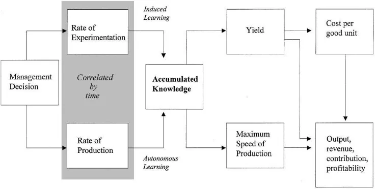
Fig. 1. Causes of learning and improvement.
aspects of problem solving for a variety of new process introductions in plants.
Zangwill and Kantor [16] point out that learn-ing can be viewed as happenlearn-ing in cycles, where the result of one cycle is the starting point for the next cycle. Each cycle can be viewed as removing some
`wastea from the manufacturing system, whether that waste is defects, causing yield loss, waste time, causing slower production, or something else such as excess inventory. This provides a very general framework in which many di!erent forms of pro-cess improvement can be modeled. As we discuss later, this cyclic model of learning"ts many aspects of ramp-up, such as the diminishing returns to experimentation in any one learning cycle. In their model, the e!ort needed for each halving of waste requires a roughly constant e!ort, giving processes which approach asymptotically to a zero-waste condition. Stata [17] provides extensive documen-tation of halving times for many kinds of waste reduction in a semiconductor company. In our models, zero waste equates to 100% yield and pro-duction at 100% of maximum theoretical speed. We show in Section 4.4 that a constant amount of experimentation is indeed needed for each halving of waste, and that it is not optimal to keep the experimentation level the same all the way through ramp-up.
Many others have looked at learning at a more aggregate level, to determine what factors drive performance improvement. These include [18}25]. Most of these articles emphasize empirical "ts to data rather than conceptual models. Mody [26] provides a model, which explicitly examines engineering e!ort as a driver of learning. Dorroh et al. [20] have a related model of make to order production, with a production function that takes knowledge and other resources as inputs. Know-ledge is produced by explicit investment in learning, independent of production. They examine the ef-fects of discounting and other parameters on the decisions of how much and when to produce and learn.
2.2. What drives learning?
Note that it may be di$cult for an outside ob-server to know whether experimentation or experi-ence is the principal driver of learning and thereby of improved performance. Both accumulated ex-periments and accumulated experience are corre-lated with time and therefore with each other. Hence, it is very di$cult to use historical data to disentangle their e!ects, especially since experi-mentation is almost never carefully tracked. There-fore, we view most of the `experience curvea
research, which purports to show that increased production leads to learning, as irrelevant to the question of what actually causes learning and how learning should be managed. In Section 5.4, we show what happens if the relative value of auton-omous vs. induced learning is over-estimated.
If experimentation is a key driver of learning, what limits the rate of experimentation? Pisano [4] points to the scarcity of production capacity during ramp-up. Many yield ramp-ups involve strenuous debates about capacity allocation between process engineers, who are measured by yield, and produc-tion managers, who are measured by short-term throughput. For example semiconductor com-panies will restrict the number of `hot lotsa, i.e. expedited engineering trials, on the grounds that such lots cause a disproportionate reduction in production and increase in service times for normal production [27]. The rate of experimentation is not the only driver of learning, of course. For one thing, theewectivenessof experimentation varies dramati-cally depending on a variety of statistical and non-statistical issues [28].
The contributions of this article are as follows. First, we analyze the interaction between capacity utilization and yields, a trade-o! of fundamental importance during production ramp-up. The model is far more detailed than any of the previous studies and thus provides a more micro-level analy-sis of ramp-up. Second, using dynamic program-ming techniques, we explicitly derive the cost and value of experimentation. These results support management in trading-o! the short term oppor-tunity cost of experimentation with the long-term value of increased processing capability. Finally, we explain a number of di!erent ramp-up patterns that can be observed in various industries and suggest which ones are best under which circumstances.
3. Yield and output during ramp-up
Our model focuses on the production ramp-up of high-tech products, such as electronics. We de"ne high-tech as meaning the company is on the cutting edge of what is currently understood in process engineering. High-tech products frequently experience high but rapidly falling prices, and the only opportunity to achieve higher than competi-tive prices is early in the product lifecycle. This forces management to bring the product to market long before the manufacturing process is fully understood. Production techniques start at low stages of knowledge and yield losses are still substantial.
During ramp-up, the goal is to raise both yield and production rate (starts per hour) as rapidly as possible. At each moment, there is a tradeo!
between the two, as the likelihood of a defect is an increasing function of processing speed. There are many causes of such tradeo!s. Consider the opera-tion of a robotic watch assembly line as described in [29]. Faster robot movement causes vibrations which decrease the precision of the assembly and thus increase the likelihood of a defect. Similar speed}precision}defect interactions occur in many automated placement and assembly operations. Similar issues apply for assembly or test operations performed by operators.
A second cause of speed vs. yield tradeo!s is rework. If there is a "xed capacity available for overall production, an increase in starts reduces the amount of capacity that can be used for rework. This reduces the number of rework loops that can be spent per defective item and thus, ultimately,
"nal yields [6].
Fourth, consider the time spent for calibration, inspection and maintenance of equipment. These operations take time, which reduces production rates. However, badly calibrated or maintained ma-chines will be more likely to produce defective parts.
Finally, many continuous and batch processes involve the application of power over time, such as baking, heat treating, and etching. The time}energy pro"le of such processes can be widely varied by adjusting temperatures, voltage, conveyor speed, and other parameters. A process can be optimized for raw speed by raising the power level and decreasing the time. However, this speed maximiz-ing settmaximiz-ing is usually not the quality/yield optimal setting, creating a tradeo!.
Each of these "ve explanations forces manage-ment to trade o!an increased level of raw through-put against production yields. In the present article, we abstract from this detailed causality and devel-op a framework that is generalizable across various industrial settings. We will "rst develop a (static) model, analyzing the interaction between capacity utilization, processing capability, and yields. This model formalizes the starts vs. yields trade-o!and is applicable beyond situations of production ramp-up. It will later allow us to show under what circumstances during production ramp-up man-agement should focus on starts or on yields (Sec-tion 3.3). In Sec(Sec-tion 4, we use the same model as the starting point for exploring the trade-o! between experiments and production.
3.1. Notation
De"ne time units such that it takes one unit of time to produce one unit of output, if the operation is executed at its maximum speed. In the presence of a speed versus yield trade-o!, it might be bene" -cial to slow down the corresponding operation by a certain timex to 1#xunits of time per unit of output. LetCbe the time available for production (e.g. machine hours) in a period. Given the de" ni-tion of time units, this also corresponds to the maximum achievable output (theoretical capacity) of the process. For a"xed`level of carea,x, chosen by management, the theoretical capacity is utilized at a percentageu"1/(1#x).
Next, we have to describe the relationship between the number of units started into the process, C/(x#1), and yields. An increase in the operation time xwill reduce the likelihood of a defect. De"ney(x,a) as the yield level as a func-tion ofx. This yield level is jointly determined by the operation timexand a parametera'0 which measures processing capability. The higher the pro-cessing capability a, the more the process can be accelerated without major yield losses:
Ly(x, a)/La'0. We assume diminishing returns of the extra operation timex, so thatLy(x, a)/Lx'0 andL2y(x, a)/L2x(0. Output is then starts times yields ory(x,a)(C/(x#1)).
Throughout the article, we assume that capacity is a binding constraint. This is characteristic of production ramp-ups since the product is still rela-tively fresh and thus in strong demand, while out-put is restricted as we will see. All units produced can be sold at a selling price p8, and the variable cost per start (e.g. raw material) isc. Before we turn to a dynamic version of the model, with learning (increase in processing capability a) or falling prices, we need to develop some simple insights about the static trade-o!between starts and yields. Looking at one period in isolation, the operation timexis chosen to maximize the contribution (sales minus variable costs), which we can write as
n(p8, a,x,c)"p8y(x, a) C
x#1!
C
x#1c.
3.2. The startsversus yields trade-ow
Good output is not necessarily a monotonic increasing function in the number of starts. Starting too many units can disturb the production process so badly that not only yields fall, but even the net number of good units produced decreases. Contri-bution falls even more than good output since the contribution measure n also takes the costs of a start into account.
To simplify analysis, we now assume a speci"c functional form for the relationship among yields, processing capability, and operation time. De"ne yields asy(x, a)"y
0(1!1/ax), which}consistent
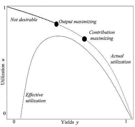
Fig. 2. Uitization versus yields (y
0"1).
with diminishing returns. The parameter y 0
cap-tures a base yield which is independent of the speed of the operation and cannot be improved, such as yield problems in operations that are downstream to the bottleneck production line. Without loss of generality, we discount the selling price by the base yields, i.e. de"nep"p8y
0. Good output per period
is now given byy
0(1!1/ax)(C/(x#1)) and the per
period contribution is
n(p, a,x,c)"p
A
1!1 axB
C
x#1!
C
x#1c.
LetxH065be the operation time that maximizes good output. It is characterized by the balance between the marginal gains from higher quality of one par-ticular unit (increased likelihood that an item started becomes good output) and the marginal losses resulting from a lower overall production rate. An additional unit started at a high level of utilization is not only likely to be defective itself, it also forces an increased processing speed on all
other items, making them more likely to be defec-tive as well. Thus, an increase in utilization is con-nected with a decrease in yields, and pushing utilization beyond uH065"1/(xH065#1) actually de-creases the overall output. At this point the e!ective capacity decreases.
In order to calculate the contribution optimal level of operation time xH#0/5, we need to take the costs per start into account, as well as the selling price. The general optimal solution is characterized by the balance between the marginal gains from higher quality of one particular unit (increased like-lihood that an item started can be sold) and the marginal losses resulting from a slower overall pro-duction. In terms of Fig. 2, this yields a downward adjustment of utilization. Thus, the contribution optimal solution has higher yields and lower utiliz-ation than the output optimal solution. We assume
p/c'1, i.e. prices adjusted for downstream yield losses are high enough to cover the variable cost of production. Proposition 1 formalizes these ideas.
Proposition 1 (Static model). The contribution opti-mal solution xH#0/5 and the output optimal solution
xH065 have the following properties:
f Both the output maximizing operation time and the
contribution maximizing operation time are strictly positive,i.e. xH065'0andxH#0/5'0.As a result of thisuH065,uH#0/5(1,which corresponds to a deliber-ate under-utilization of the capacity.
f The output maximizing operation timexH
065and the
corresponding contribution levelPH
065are given by
xH065"1#J1#a
a ,
PH
065"n(p,a,xH065,0)
"Cp 1
1#(2/a)(1#J1#a). (3.1)
f The contribution maximizing operation time xH #0/5,
the corresponding yield level y(xH#0/5, a), and the resulting contribution levelPH
#0/5 are given by
xH#0/5"1#J1#a!ca/p a(1!c/p) ,
yH#0/5"y(xH#0/5, a)"J1#a!ca/p#c/p
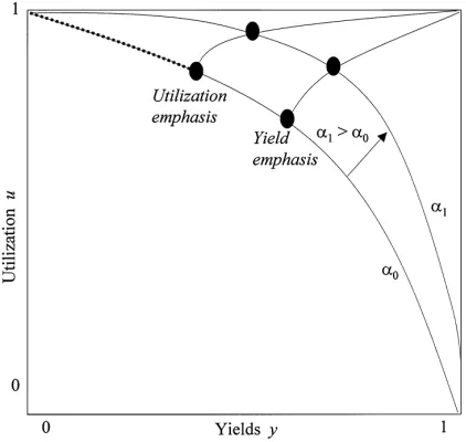
Fig. 3. Increasing processing capability: the ramp-map (y
0"1).
PH
#0/5"n(p, a, xH#0/5,c)
"Ca(p!c)2
p
1
2J1#a!ca/p#2#a!ca/p.
f The contribution maximizing operation time xH#0/5 decreases with the selling price p being in-creased relative to cost c(p/cincreases).For large
values ofp/cthe contribution optimal solution ap-proaches the output optimal solution:xH#0/5PxH065.
Proof. For easier readability, all the proofs are given in the appendix.
The"rst part of Proposition 1 shows the di! er-ence between utilization and e!ective utilization: it is both contribution and output optimal not to operate the production line at its maximum speed. Pushing utilization aboveuH065 is not bene"cial, as the yield losses more than o!set the gains from starting more units. At this point, the e!ective util-ization of the plant is maximized.
Proposition 1 also shows how the optimal opera-tion times xH#0/5 and xH065 depend on the various parameters, especially the processing capabilitya. Yields and contribution can also be written as functions ofa. The last point in Proposition 1 states that a decrease in selling pricepwill}everything else equal } reduce the number of starts and in-crease the resulting yields. Thus, with falling prices, the production line needs to put an even higher emphasis on quality.
Finally, it is interesting to observe the di!erence between (3.1) and (3.2). For the special case where the cost per startc"0, the two are identical. For
c'0, utilization is adjusted downwards in favor of yields. This con"rms the intuition generated by Fig. 2. Thus, a simple corollary of Proposition 1 is thatyH065)yH#0/5 and, for the corresponding utiliz-ation levels,yH065)yH#0/5.
3.3. Yield emphasisversusvolume emphasis
Consider a sequence of periods similar to the one described above. The only di!erence between each period is the processing capabilitya: over time, the organization learns more about its production pro-cess, which corresponds to an increase ina. Note
that an increase inaallows for higher yields at the same level of starts, or more starts at the same level of yields. In this section, we are not explicit about
how the learning occurs. It might be driven by volume, by an organizational learning e!ort, or by time alone.
The result of these changes is a sequence of models similar to the static model described above. This constitutes the "rst step toward a `dynamic ramp-up problema. A natural question to ask in this model is: What should the plant do with its increased processing capabilities, produce more or further increase yields (at the cost of output)? To illustrate this trade-o!, we extend Fig. 2 by showing various levels ofa. Each of the points on the addi-tional lines corresponds to a pair of yield and utilization level, i.e. a set of (yH
t,uHt), that is
com-puted using (3.2) for a changing level of processing capabilitya. We de"ne this path of utilization/yield combination as the ramp-map. This is summarized in Fig. 3. Let ayield-emphasizing rampbe a ramp with high initial yields (relative to utilization,uH/yH
Proposition 2 (Ramp-map). If learning occurs exogenously to the model, i.e. the operation times
x
thave no impact on any futureai,then the ramp-map has the following properties:
f Long-run behavior: for aPR, yHPy 0 and uHP1and as a resultuH/yHP1/y
0.
f For smalla,uH/yHis an increasing function inp/c.
Largevalues ofp/cfavor a utilization emphasizing ramp.
f For large values of p/c, uH/yHPuH 065/yH065
"a/(1#a)y
0,which characterizes the maximum
possible utilization emphasis. The ramp-map above this path is empty.
Proposition 2 is interesting in several ways. First, we see that regardless of cost per startcand selling pricepthe long-run behavior for increasing levels of processing capability ais always perfect yields (yHPy
0) and 100% utilization (uHP1). This
pro-vides the end-point of the ramp-map. Second, the ratiouH/yHhelps us to further specify the location of the start-point. For large ratios of price to cost
p/c, following Proposition 1, the only focus is on output, thusuH/yHis maximized. At this point, the ratio between utilization and yields is characterized bya/(1#a). For smaller values ofp/c, there is an extra focus on yields, which means the path through the ramp-map shifts to the lower right.
To illustrate the implications for di!erent indus-trial processes, compare disk drive assembly and semiconductor wafer production. For drives, the costs of raw material are very close to the market price of the"nished good, which makes scrapping a drive extremely expensive. Even if"rst-pass yields are low, rework is used intensively to reach high
"nal yields. Rework corresponds to an extended operations time, x
t, in our model. Proposition
2 predicts a strong yield emphasis in the ramp-up, which is consistent with empirical research in this industry [6].
For semiconductors, the main cost driver is the equipment, rather than the raw material. Thus, the value of the"nished wafer is many times its cost per start and scrapping a defective wafer loses little in terms of direct cost. Following Proposition 2, the main focus is on output and the ramp-up is charac-terized by extremely low initial yields. Various
studies in the semiconductor industry show that production can sometimes continue at low yields for a prolonged period, if competition is low and prices high (e.g. [11]).
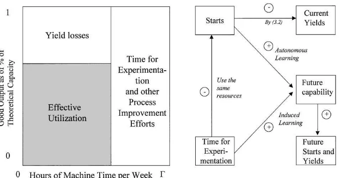
4. Learning in ramp-up
In this section, we extend our analysis presented in Section 3 by explicitly modeling the sources of learning. We do this by adding a second managerial decision variable, learning e!orts, which will come in the form of controlled experiments. The results of Proposition 1 allow us to replace the decision vari-able `operations timea, x
t, with its contribution
optimal level xH#0/5 and thereby to focus our discussion purely on learning e!orts.
The bene"t of learning e!orts lies in an increased knowledge about the production process, which is captured in the processing capability parameter
ain the model. However, learning also has draw-backs. First, experiments consume capacity which could otherwise be used for regular production (e.g. setups of experiments, experimental output might not be salable, disruption from expediting experi-mental`hot lotsa). Second, experiments are a devi-ation from what is currently believed to be the optimal process control. This lowers yields (e.g. in case of trying out a new recipe).
This creates a dual role of the production pro-cess: it not only produces salable output, it also provides the environment for conducting experi-ments [28]. Looking at the per period contribution
PH
#0/5in (3.2), we see that the overall contribution is
proportional to the available capacityC. So,
spend-ing more machine time for experimentation creates an opportunity cost of lost regular production.
Fig. 4. E!ects of experimentation.
2This formulation of learning is equivalent to assuming j"cz
1c1~2 z, wherec1 is de"ned as the absolute importance of
learning by experimentation andc2as the absolute importance of learning by doing.
producers of knowledge as well as of productsa. These con#icting goals and their interaction are illustrated in Fig. 4.
4.1. A mathematical model
In order to formalize the tradeo! between cur-rent production and learning, we de"ne z as the fraction of the overall processing capacityCthat is
used for experiments. Together with the operations time (level of care) x, the experimentation time represents our second managerial decision variable. The overall output of the production process is then
(1!z)y(x,a) C
x#1, where 0)z)1.
Process improvement corresponds to an in-creased value of processing capabilitya. Consider the case where we improve the process by increas-ing the processincreas-ing capability froma0-$ to a higher level a/%8:"ja
0-$'a0-$. The magnitude of the
improvement j from one period to the next will depend on the two learning mechanisms, learning by doing and learning by experimentation. Similar to a production function, we assume
j"bz 1b2,
whereb1captures the relative importance of learn-ing by experimentation to learnlearn-ing by dolearn-ing and
b2the learning rate of learning by doing in itself.2
In the absence of experimentation (z"0), process improvement is solely a result of learning by doing (j"b
2). Learning by doing is thus driven by the
cumulative time (e.g. machine hours) the produc-tion line has been processing the new product.
b1measures how much additional progress would occur if the line were dedicated to experiments for thewholeperiod.
We now extend our static model of Section 3 to a¹-period dynamic model. The previously intro-duced variablesa,xandpfor processing capability, operations time, and price are now indexed by time, i.e. a
t,xt and pt. Over the periods, prices fall at
a rate ofd1 per period, and future cash#ows (rev-enues and cost) are discounted with a factord$. As this paper focuses on the dynamicsinsidethe plant, we view this price fall as exogenous to our model. In every period, management needs to decide on both speed of the line (in form of the operations timex
experi-mentation z
t. Whereas the costs of an experiment
are additive over time (the"rst 10% of production capacity has the same opportunity cost as the last 10%), the value of an experiment typically is not. For example, spending 20% of the capacity for experimentation in one period will yield a smaller increase in processing capabilitya
t than spending
10% in the current period and 10% in the sub-sequent period.
There are several reasons for diminishing returns to experimentation within one period. First, experi-mentation is normally done in cycles, rather than in one single batch [16]. It is more e!ective to wait for the results of one experiment before formulating ideas which become the basis of the next cycle [30]. Second, although capacity is a key input for experi-mentation, there are others, speci"cally engineering time. Third, conducting too many experiments at the same time increases the noise in the process, which makes it harder to learn. Thus, process im-provement returns will be reduced, if management decides to`jamaall experimentation e!orts in one or few periods.
To capture these diminishing returns to mentation, we adjust the learning rate of experi-mentation b1 by multiplying it with a factor Hz, which is decreasing in the amount of experimenta-tion, z, carried out in that period (H(1). This reduces the e!ective learning rate of experimenta-tion to b1Hz, and therefore results in an overall process improvement of
j": b2[b1Hz]z"bz1Hz2b
2. (4.1)
For small values of experimentation time z, the factor Hz is close to one, i.e. for the "rst units of
experimentation, the marginal gains are close to the ideal learning rate b1. In the extreme case of
z"1, only H percent of the ideal learning rate is
achieved. immediately that the e!ect ofHis minimized if the experiments are evenly spread over the periods. Therefore, if cost and value of the experiments were constant over time, it would be optimal to have
z
1"z2. However, in the presence of changing cost
and value, the optimal solution has to be chosen based on the overall optimization problem.
4.2. Dynamic programming formulation
As the operation time x
t has no e!ect on any
future processing capabilitiesa
t`i, i"1,2,¹!t,
we candecompose the overall optimization prob-lem. For every period, we choose the optimal op-eration timexH#0/5given current capabilitya
t, which
is given by Proposition 1. Anticipating that we will choose this optimal operation time, we then are left with"nding the optimal learning e!ortz
tfor every
period. This requires the analysis of a dynamic program with the processing capability at as the state and the experimentation levelz
t as the
deci-improvement rate given in (4.1) and the immediate pay-o!s per period are de"ned as
For the last period ¹, there is no direct value of experimentation in our model. However, higher processing capability beyond period ¹ typically has some value, e.g. in lower unit costs for the residual product lifecycle or in increased knowledge for future product generations. For a general periodt, we can see from (4.3) that the"rst part of
F
t(at) is decreasing linearly in the experimentation
time z
t. As we will show more formally below,
the returns to experimentations are marginally decreasing, which makes (4.3) a sum of two concave functions. Thus, the optimal solutions zH1,2,zHT
are uniquely identi"ed and can be computed by backward induction.
4.3. Costs of an experiment
"rst sight, the analysis looks quite simple: costs of experimentation are given by the opportunity costs of not producing and the bene"ts of experimenta-tion are given by the increased process knowledge that we have already formalized in (3.2).
Although this intuition is correct, the actual analysis is more complicated, as both opportunity cost and value of increased process knowledge are functions of time and current processing capability. Time is important as it relates to selling price and thus to the opportunity cost of not producing. The current knowledge is important as it in#uences how much is still to be learned from an experiment as well as the opportunity cost. Having the line not produce is cheaper at a low level of knowledge than at a high level of knowledge.
Letk(t, a
t,zt)"MaxMztnt(at), 0Ndenote the cost
of experimentation if a fraction z
t of capacity is
used for experimentation at timetand statea
t. We
can then prove the following proposition.
Proposition 3a (Cost of an experiment). The cost
k(t,at,z
t)of doingztunits of experimentation in time
tand stateat is an increasing function of the process-ing capabilitya
t,and a decreasing function of timet.
Proposition 3a means that the cost of experi-mentation can, over the periods 1,2,¹, go either
up or down. Increasing levels of processing capabil-itya
t bring the opportunity cost up, as at a high
a the production line can produce more and at higher yields. However, falling prices, which also drive the opportunity cost, are pushing the oppor-tunity cost down. As over time the organization increases its processing capability, at and t move together, allowing the cost of experimentation to go either up or down.
Before we turn to the value of an experiment, we compute the costs of increasing the processing ca-pability froma
t tojat`1. This extends Proposition
3a which derived the costs of experimentation per unit of experimentation time.
Proposition 3b (Doubling a). Increasing the pro-cessing capability by a factorjcarries the following costs:
f the amount of experimentation required as a
func-tion ofjis given by
We can see that although the required amount of experimentation to increase the processing capabil-ity from ato ja is independent of time, the asso-ciated costsk(t,at,z(j)) are not. This is a result of Proposition 3a. Eq. (4.4) shows the relationship between experimentation time and the learning parametersb1,b2, andh. These parameters provide an upper bound of how much improvement can be achieved within one period. We can see that a doubling of the processing capabilityabecomes more and more expensive asaincreases, and has to be justi"ed by large bene"ts. These bene"ts are now analyzed in greater detail.
4.4. Value of an experiment
The value of an experiment depends on three factors: how far the product has advanced in the lifecycle (the periodt), the current processing capa-bilitya, and the level of experimentationz. Similar to the cost of an experiment, both timetand pro-cessing capabilitya(the two state variables of the DP) have an in#uence on the value. The value of a unit of experimentation depends on how much additional experimentation is conducted in that particular period. We de"nev(t, at,z
t) as the value
of doingz
t units of experimentation in timetand
statea
t units of experimentation will bring the
processing capability at period t#1 from a
t to
a
tbz1tHz 2
tb
2. The net present value of this is given by F
t`1(atbz1tHz 2
tb
2). If we decide to not invest into
process improvement, the new state will be a
tb2
with the associated net present value ofF
t`1(atb2).
the net present value di!erence between two scen-arios, corresponding to two di!erenta-trajectories, starting at periodt#1. The"rst scenario is based on optimal experimentation in periodt, the second scenario forcesz
t"0. Note that the two scenarios
are likely to have di!erent experimentation policies beyond periodt#1.
Proposition 4 (Value of experiment). The value of increasing the processing capability fromatojagoes down in a (diminishing physical returns) as well as int.
Proposition 4 shows the value of an experiment falls over time. There are three reasons for this. First, the residual lifetime of the product, to which the new knowledge might be applied, is shrinking. Second, the value of an experiment falls as prices fall. This makes early knowledge more valuable than late knowledge.
Third, in addition to those two e!ects, that are purely driven by calendar time, the value of an experiment falls as a increases. To illustrate this, compare two situations. In the "rst situation, the processing capabilityais small and yield losses are still high. Increasingaat this point has substantial leverage, as there are still plenty of opportunities for improvement. In the second situation, the pro-cess is close to being perfect. Both utilization,u, and yields,y, are close to one, so an improvement ina, even if of substantial size, will not have much im-pact on the bottom line.
This is similar to the argument of Zangwill and Kantor [16]. Instead of looking at process yields, they make waste (de"ned as 1-yields) their key variable. The authors argue that the e!ort required for a proportional waste reduction is constant. For example, getting yields from 50 to 75% and getting them from 75 to 87% both correspond to a halving of waste, and require the same e!ort, but the"rst improvement is more valuable then the second. This is consistent with our model, if we de"ne waste as 1/ax, and Proposition 3b, which requires a con-stant e!ort for each proportional change ina. Thus, there exists a constanta-improvement (in form of a multiplier) for each halving of waste.
We now turn to a series of numerical examples, which illustrate how qualitatively di!erent optimal
behavior can arise from di!erent market, technolo-gical, and learning parameters.
5. Numerical illustrations
We solve a number of numerical examples in this section. They shed light on the structure of the optimal solution to the general pro"t maximizing problem as stated in (4.2). Consider an example of a low price to cost ratio process, such as disk drive assembly. The initial price isp"$3/unit, prices fall atd1"0.95 per period (month), the discount factor is d$"0.98. We assume cost per start to be
c"$1/unit and consider only the"nal assembly, so there are no substantial yield losses further down-stream (y
0"1). Let the initial processing capability
bea1"1 and the learning rates beb1"2.80 and
b2"1.01 for learning by experimentation and learning by doing respectively. The overall capacity available for production and experimentation is
C"1000 units per month, and the lifecycle is
¹"12 months.
5.1. High experimentation capability
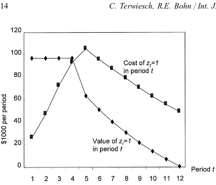
To begin with, consider the case where the ex-perimentation capability is high, i.e.h"1. Engin-eers can conduct a large number of experiments and still get the maximum learning out of each of them. We can compute the cost of an experiment in the"rst period using Proposition 3a. With no ex-perimentation, the optimal "rst period pro"t is
n1"25.4. Thus, each percent of experimentation time creates an opportunity cost of
k(1,a1, 0.01)"0.254. The value of experimenta-tion is driven by the future periods' increased capability.
Fig. 5. Cost and value (in dollars) of experimentation.
3Note that these values are`not realizeda, as the complete
"rst periods are dedicated to experimentation.
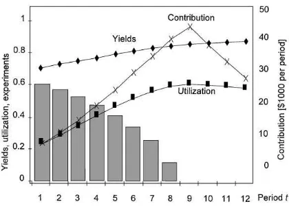
Fig. 6. Optimal solution for h"1; the bars indicate the optimalz
t.
in connection with Proposition 4. First, there are fewer periods left to which the additional know-ledge can be applied. Second, because of the physical diminishing returns, a further increase in processing capability has less value.
As a result, no time is spent on experimentation in the fourth period and beyond. Fig. 5 also shows that experiments are inexpensive in the beginning and in the end of the product lifecycle, but most costly in the middle.
Fig. 6 summarizes the optimal solution. The four bars indicate the optimal experimentation policy: full experimentation at the start, then none. Fig. 6 also shows yields, utilization, and per period contribution. We see that the initial focus of the plant is on yields (start at 72%) rather than utiliz-ation (start at 26%).3This yield emphasizing ramp is a result of the relatively small price to cost ratio (initially 3 : 1).
5.2. Low experimentation capability
Next, consider the case of lower experimentation capability, e.g.h"0.5. The cost per unit of experi-mentation is the same in the "rst period, but its value goes down drastically. Spendingz
1"1 units
on experimentation now only results in a second
period capability ofa2"1.46. This is driven by the sub-additivity argument. The lower a2 also translates into a lower second period opportunity cost of the coming periods (k(2,a2, 0.01)"0.31,
k(3,a3, 0.01)"0.36,k(4,a4, 0.01)"0.40). The de-crease in k(2,a2, 0.01) together with the reduced
"rst period value of experimentation creates an incentive to move some experiments from period one to period two.
Fig. 7 shows the optimal solution for the case
h"0.5. Again, the emphasis of the ramp is on yields, rather than utilization. As opposed to the previous example (and Fig. 6), production starts in the"rst period, so the plant is actually producing at the initial yields of 72%. Fig. 7 demonstrates the harsh economic reality that most companies face during ramp-up. Given its low learning capability captured inh"1
2, it is not until period 9 (75% into
the lifecycle) that the plant reaches its maximum contribution. However, rapidly falling prices quickly erode even the remaining 25% of the lifecycle, so that the time that can be used to pay back development expenses is extremely short.
These "rst two examples have illustrated the importance of the sub-additivity parameterh. The
Fig. 7. Optimal solution for h"12; the bars indicate the optimalz
t.
several periods. Although this approach allows for some early pro"ts and high prices, it also forces management to run the production line at low yields and utilization. As expected, the overall pro"t in the "rst example (n"522.5) exceeds pro"ts in the second one (n"296.3).
5.3. Rapidly falling prices
Next, consider a situation of rapidly falling pri-ces. Suppose R&D has come up with a radical new product that is the "rst of its kind. For the "rst period, we can charge a monopoly price of p"5. Afterwards, competitors enter the market and pri-ces drop sharply top"3, and from then onwards fall atd1"0.95. All other parameters are identical to the second example above. This example is inter-esting as it demonstrates that the capacity dedi-cated to experimentation should not necessarily decrease over time. The cost of experimentation in the optimal solution are given by
k(1,a1, 0.01)"0.58 and k(2,a2, 0.01)"0.28. Compared to the second period, prices are high in the "rst period, which drives up the opportunity cost of not producing. The initial processing capa-bility a1"1 is su$ciently high to create pro"ts. This picture changes in the second period. As little time was spent on experimentation in the"rst peri-od,a2"1.39, which is not a substantial increase. However, given the drastic fall in prices, manage-ment now faces a situation where the selling price is
substantially lower than before. This price level together with the current processing capability makes experimentation now less expensive, yield-ing a second period experimentation ofz
2"0.57.
From then onwards, the cost of experimentation follows the path we have seen in the"rst two cases: an initial increase because of the increased capabil-ity and a long-term decrease because of falling prices. The optimal level ofz
2 toz12 is decreasing
in time.
Taking the above examples together with Prop-ositions 3 and 4, we can postulate three types of solution:
1.Virtual pilot line: The introduction of the prod-uct is delayed and all available capacity is used for experimentation (zH
t"1 fort"1,2,n(¹). This
approach is optimal if (a) prices are falling at a modest rate (d1is low), (b) high experimentation capability (weak sub-additivity:his close to 1).
2. Mix of experiments and production: Experi-ments are spread out over several periods, but more and more of the production capacity is used for regular production (z
t'zt`1'0). This approach
is optimal for low experimentation capability. 3. Delayed experimentation: The time spent for experimentation is larger in the second period than in the"rst period (z
2'z1'0). This approach is
optimal if prices fall faster in the beginning than they do later.
5.4. Knowing the sources of learning
The above examples assume that management is fully aware of the true sources of learning. This includes both the relative magnitude between
learning and speci"cally underestimates the im-portance of learning by experimentation.
Consider a situation similar to the example of Section 5.1. The initial processing capability is
a1"1 and the learning rates are b1"2.8 and
b2"1.01. However, these underlying parameters are not known by managers, who have estimates of the learning rates in form ofbK
i,i"1, 2. LetbK1"2
andbK2"1.5, which corresponds to an overestima-tion of experience versus experimentaoverestima-tion. Based on this assumption, management chooses the ex-perimentation times to maximize lifecycle contribu-tion according to (4.2). This yields lower than optimalz
t and a total contribution of n"235. If
management had followed the true optimal policy the discounted contribution would have been
n"296. In other words, 20% of the potential con-tribution is lost because of an incorrect estimate of the learning rate.
Next, consider the reverse case where the real learning rate is b1"2.8, however engineering over-estimates the importance of experimentation, withbK1"5. As a result of this, more time is allo-cated to experimentation than optimal. Instead of getting a contribution ofn"296, the product now only reaches contributions ofn"267.
Two remarks clarify these examples. First, in both of them management was aware that experi-mentation yields higher improvement rates than pure volume, but the magnitude of these rates were misestimated. If management thinks the only source of learning is regular production (`learning by doinga), no time will be spent on experimenta-tion (z
i"0). The resulting loss of contribution is
even larger than in the two examples.
Second, a deviation of 10}20% innseems to be relatively small, especially if compared to how far the bKi estimates were from the true values. How-ever, this is looking at contribution, rather than pro"ts. In presence of large"xed costs, a 10}20% contribution change will make the di!erence be-tween bottom line pro"ts and losses.
6. Conclusion,implications and future research
We have presented an analytical model of pro-duction ramp-up, which combines a static trade-o!
between yields and utilization with a dynamic trade-o!of learning and process improvement. In today's rapidly changing environments, cutting de-velopment times (time-to-market) in itself is not su$cient. Another key to achieving high pro"t is a rapid production ramp-up of a new product. This includes quickly achieving both high yields and a high level of utilization.
Our "ndings have a number of managerial im-plications. Most basic is the need for managers to accept and deal with the inherent paradox of learn-ing durlearn-ing production ramp-up. At the beginnlearn-ing of a ramp when prices are at their highest, and yields and output at their lowest, it is nonetheless still the moment to further reduce output in order to run engineering trials and work on yield and speed improvements. This paradox often creates, in our experience, strong pressures to take shortcuts in learning, such as experiments with overly small sample sizes relative to the process noise level, or not running validation trials before implementing process changes. While this keeps up-time higher in the short run, it often leads to problems which reduce performance for the rest of the ramp-up period and beyond. We deal with this paradox by explicitly calculating the cost and value of experi-mentation as functions of time and processing ca-pability. Figs. 6 and 7 show the patterns that can result from optimal behavior.
Second, we show the importance of understand-ing the sources of learnunderstand-ing. It is incorrect to treat learning as an exogenous process beyond manage-rial control. Rather, there are three key high-level inputs which should be explicitly allocated and managed. These are normal production experience, capacity withdrawn from production for experi-ments of many kinds, and engineering time. Only the"rst of these happens automatically. Only en-gineering time (which we modeled as being lumped together with experimentation) appears explicitly in a cost accounting system. But the dollar costs of experimentation time, although not captured in accounting systems, can be a large investment as well, and are integral to success.
care and rework shift. It also serves as a strong reminder that in yield driven industries there is a large di!erence between utilization and e!ective utilization. Finally, this research illustrates the im-portance of time-to-volume compared with the still dominant paradigm of time-to-market. We show how di!erent situations require di!erent decisions during the ramp-up period.
We have kept the model as simple as possible in order to focus on structural results. This approach clearly has limitations. Our assumptions that the processing capability can be represented as a single number, as well as the assumptions concerning the functional forms of learning rates and sub-additiv-ity are strong simpli"cation of real ramp-up situations. Re"nements of the model provide inter-esting avenues for future research. First, some of the assumptions could be relaxed. For example, prices and competitive behavior could be explicitly modeled. Spence [31] provided an in#uential analysis of the e!ect of learning on strategic competition. He modeled a"rm investing in learn-ing early, in order to deter entry by potential competitors. In his model, learning was an inherent by-product of production experience, so that the form of `investmenta was to produce more. The
"rm uses low prices both to encourage demand, and to serve as a signal to competitors that it has made an investment. This leads to the prescription to `price ahead of the learning curvea. In our model,"rms can also invest in learning, but in the form of deliberate learning through more time for experiments (andlessproduction). A combination of both models seems promising.
Second, we see a strong need for more empirical research on this topic. Detailed case studies on the ramp-up period will help to reveal addi-tional variables [32]. Such case studies could try to develop a managerial check-list of items that need to be addressed before or during the ramp-up. Another empirical research opportunity lies in a detailed econometric analysis of yield and utiliz-ation curves over time, which tries to identify the most e!ective variables that help increase the e!ective capacity.
Finally, the issues of production ramp-up should be linked to the existing"elds of product develop-ment and learning in manufacturing. Although in
the present paper we try to explicitly include" nd-ings from the manufacturing learning literature, we do not su$ciently include aspects of product devel-opment. What happens during product develop-ment will have a strong impact on the initial processing capability as well as on the speed of up. Thus, linking the quality of the ramp-up to events during the product development process provides a third interesting avenue for future research.
Appendix. Proofs of Propositions 1}5
Proof of Proposition 1. We need to show that there exists both a unique output maximizing care timexH065 and a unique contribution maximiz-ing care timexH#0/5. To do this, we uses"C/(1#x) and show that there exists a uniquely de"ned optimal levels of starts. Given the 1 : 1 trans-formation between s and x, this also uniquely characterizes the optimal care levels xH065 and
xH#0/5. Output as a function of starts is given by
q(s)"s(1!(1/a)(1/C/(s!1)). As L2q(s)/L2s" !2!4(s/a(C!s))!2s2/(a(C!s)2)(0,q(s) is concave in s. The contribution maximizing prob-lem can be restated as pq(s)!csPMax, which provides a linear combination of concave functions, and thus itself is concave.
Thus, bothxH065 and xH#0/5 can be obtained from
"rst-order conditions and the corresponding yield and contribution levels result from substituting
xH065 and xH#0/5 into the corresponding de"nitions. Eq. (3.2) converges to (3.1) for largep(c/pP0). h
Proof of Proposition 2. As uH"1/(1#x), with
aPR, we can see from (3.2) thatxP0 and thus
uHP1. The same holds for yields yH.
The ratio uH/yH indicates to what extent the process focuses on output or yields. From Proposition 1, we can determine
uH
yH"a (p!c)
p
1#J1#a!ca/p
All of the proposed statements can be derived from the ratiouH/yH. h
Proof of Proposition 3. Proof(3a): We can see from Proposition 1 thatn
t(at) is increasing withat, as the
operation time (3.2) decreases with a(thus a high
a allows for more starts) and the corresponding yield level also increases witha.
To show that costs are decreasing withp
t, de"ne
where, without loss of generality, c"1. As
p'c"1, the second derivative is positive (i.e. costs are falling). This is, holding a
t constant, the
only parameter changing with time.
Proof (3b): Eq. (4.4) can be derived by solving
ja"abz
1Hz2b2 for z. After taking logarithms,
we obtain a quadratic expression in z, yielding two solutions. As j has to be smaller than
b1b2H, which is the maximum achievable improvement (z"1), the optimal solution is given by (4.4). h
Proof of Proposition 4. To establish the diminish-ing returns we de"nemas above and compute
L2PH derivative is (0 which shows that PH
#0/5 grows
slower for large values ofa.
First, prices are falling over time, and second, the residual lifetime to which the new knowledge can be applied is shrinking. Each of the two arguments is su$cient in itself to make the value of an im-provement go down int. h
References
[1] R.J. McIvor, D. Martin, H. Matsuo, J. Ng, Pro"ting from process improvement in the new semiconductor manufac-turing environment, Technology and Operations Review 1 (2) (1997) 1}15.
[2] J. Dutton, A. Thomas, Treating progress functions as a managerial opportunity, Academy of Management Review 9 (2) (1984) 235}247.
[3] S. Thomke, Project dreamcast: Serious play at Sega Enter-prises Ltd, case study N9-600-028, Harvard Business School, Boston, 1999.
[4] G. Pisano, The Development Factory, Harvard Business School Press, Boston, 1995.
[5] R.E. Bohn, Measuring and managing technological know-ledge, Sloan Management Review 36 (1) (1994) 61}73. [6] R.E. Bohn, C. Terwiesch, The economics of yield-driven
processes, Journal of Operations Management 18 (1999) 41}59.
[7] N.S. Langowitz, An exploration of production problems in the initial commercial manufacture of products, Research Policy 17 (1988) 43}54.
[8] R.H. Benfer, Learning during ramping: Policy choices for semiconductor manufacturing "rms, M.S. Thesis, MIT, Cambridge, MA 1993.
[9] R.T. Clawson, Controlling the manufacturing start-up, Harvard Business Review 63(3) (1985) 6}20.
[10] N.H. Wasserman, K.B. Clark, Everest Computer, case study 685-085, Harvard Business School, Boston, 1986. [11] R.C. Leachman, Competitive semiconductor
manufactur-ing survey: third report on the results of the main phase, Berkeley Report CSM-31, 1996 (Chapter 2).
[12] J.M. Dutton, A. Thomas, J.E. Butler, The history of pro-gress functions as a managerial technology, Business His-tory Review 58 (2) (1984) 204}233.
[13] L. Argote, D. Epple, Learning curves in manufacturing, Science 247 (23) (1990) 920}924.
[14] M.A. LapreH, A.S. Mukherjee, L.N. Van Wassenhove, Be-hind the learning curve: linking learning activities to waste reduction, Management Science, forthcoming.
[15] E. von Hippel, M.J. Tyre, How learning is done: problem identi"cation in novel process equipment, Research Policy 24 (1) (1995) 1}12.
[16] W.I. Zangwill, P.B. Kantor, Toward a theory of continu-ous improvement, Management Science 44 (7) (1998) 910}920.
[17] R. Stata, Organizational learning}the key to manage-ment innovation, Sloan Managemanage-ment Review 30 (1989) 63}74.
[18] P.S. Adler, Shared learning, Management Science 36 (8) (1990) 938}957.
[19] P.S. Adler, K.B. Clark, Behind the learning curve: A sketch of the learning process, Management Science 37 (3) (1991) 267}281.
[21] D. Epple, L. Argote, K. Murphy, An empirical investiga-tion of the microstructure of knowledge acquisiinvestiga-tion and transfer through learning by doing, Operations Research 44 (1996) 77}86.
[22] H. Gruber, The yield factor and the learning curve in semiconductor production, Applied Economics 26 (1994) 837}843.
[23] K. Mishina, Learning by new experiences: Revisiting the
#ying fortress learning curve, in: N. Lamoreaux, D. Ra!, P. Temin (Eds.), Learning by Doing in Markets, Firms, and Countries, University of Chicago Press, Chicago, 1998.
[24] M.A. LapreH, L.N. Van Wassenhove, Productivity improve-ment in a network of learning factories: A learning curve analysis, Working paper 98-02, BU School of Manage-ment, 1998.
[25] A.S. Mukherjee, M.A. LapreH, L.N. Van Wassenhove, Knowledge driven quality improvement, Management Science 44 (11) (1998) 35}44.
[26] A. Mody, Firm strategies for costly engineering learning, Management Science 35 (4) (1989) 496}512.
[27] B. Ehteshami, R.G. Petrakian, P.M. Shabe, Trade-o!s in cycle time management: Hot lots, IEEE Semiconductor Manufacturing 5 (2) (1992) 101}106.
[28] R.E. Bohn, Learning by experimentation in manufactur-ing, Harvard Business School, Working paper 88-001, 1987.
[29] R. Jaikumar, R. Bohn, A dynamic approach to operations management: an alternative to static optimization, Inter-national Journal of Production Economics 27 (3) (1992) 265}282.
[30] C.H. Loch, C. Terwiesch, S. Thomke, Parallel and sequen-tial testing of design alternatives, Working Paper at The Wharton School, Harvard Business School, INSEAD, 1999.
[31] M. Spence, The learning curve and competition, The Bell Journal of Economics 12 (1981) 49}70.