Herbert Stahl
†Abstract
The convergence of (diagonal) sequences of rational interpolants to an an-alytic function is investigated. Problems connected with their definition are shortly discussed. Results about locally uniform convergence are reviewed. Then the convergence in capacity is studied in more detail. Here, a central place is taken by a theorem about the convergence in capacity of rational in-terpolants to functions with branch points. The notion of a symmetric domain plays a fundamental role. Apart from very special situations, proofs of the existence of such domains are known so far only for two types of interpolation schemes.
1
Rational Interpolation
Interpolating and approximating an analytic function by polynomials or rational functions with prescribed poles is rather well understood and has been studied in great detail by J.L. Walsh (cf. his book [Wal]). In many respects interpolation by rational functions with preassigned poles leads to a theory very similar to that of polynomial interpolation. A rather different situation arises if one considers inter-polation by rational functions with free poles. Free poles means here that both, the numerator and the denominator polynomial, are determined by the interpolation conditions, while in case of preassigned poles this is true only for the numerator polynomial. The theoretical background of rational interpolation with free poles is very similar to that of Pad´e approximants. Actually, Pad´e approximants are a special type of rational interpolants, they are linearized (also called generalized) rational interpolants with all its interpolation points identical. In the literature ra-tional interpolants with free poles are also known under the name of multi-point Pad´e approximants. There are good reasons for this somewhat strange terminology. Problems connected with the definition of rational interpolants will be addressed in the next paragraphs.
∗Research supported by the Deutsche Forschungsgemeinschaft (AZ: Sta 299/8–1). †Dedicated to Jean Meinguet on the occasion of his 65th
anniversary 1991Mathematics Subject Classification : 41A20, 41A25, 30E10.
Contrary to the situation in polynomial interpolation, for rational interpolation there is no definition that satisfies all wishes a potential user naively could have; some compromises are always necessary, and they result in a definition that may surprise at first glance. The definition will be discussed in the present section. The material is based on the excellent survey paper [Me] by J. Meinguet, which covers many other aspects of the problem including a very interesting and detailed review of the historic development.
Let an infinite triangular matrix of interpolation points aij ∈C (called
interpo-lation scheme) be given:
of the matrixAdefines aninterpolation set withn+ 1 interpolation points. It is not excluded that some or all points are identical. Hence, in (1.2) we have in general a multiset with multiplicities of elements taken account of by repetition. With each interpolation set An a polynomial
By f we denote the function which will be interpolated. In the sequel it is assumed that this function is analytic at each point z ∈ An, n ∈ N. By Pn and
Rmn we denote the set of all complex polynomials of degree at most n and the
set of rational functions of numerator and denominator degree at most m and n, respectively.
Remarks: (1) Condition (1.4) implies that at each zero of the polynomial wm+n
the interpolation errorf−rmn has a zero of at least the same order. Thus, f−rmn
has a zero at each pointx∈Am+n of at least the same order as the frequency of the
point x in the set Am+n, or in other words, the interpolant rmn and its derivatives r(k)
mn coincide with the function f and its derivatives f(k) at the point x up to an
order determined by the frequency of x in Am+n. Relation (1.4) therefore defines
interpolation in Hermite’s sense.
(2) As the next example will show, the existence of a rational functionrmn ∈ Rmn
exists that satisfies (1.4), then one says that the Cauchy interpolation problem is solvable (cf. [Me], Introduction).
(3) If the interpolation problem is solvable, then the solution is unique, which can easily be verified by comparing two potential candidates.
Example 1.1: We choose m = n = 1, A2 := {−1,0,1}, and as function to
be interpolated f(z) := z2. Any rational function r ∈ R
1,1 is either a Moebius
transform or a constant. Ifr is a Moebius transform, then it is univalent in C and
therefore cannot interpolate the value 1 at the two different points−1 and 1. Ifris a constant function, then it cannot interpolate the two different values 0 and 1. Hence, already in this very simple situation a rational functionr1,1(f, A2;·) satisfying (1.4)
does not exist.
Comparing rational interpolation with interpolation by polynomials, or by ele-ments of any other family of functions forming a Chebychef systeme, shows that the main reason for the non-existence in case of rational interpolants is caused by the non-linearity of the parametrisation of the interpolants. In order to circumvent the difficulties one uses a linearized version of Definition 1.1. Actually, this has al-ready been done by Cauchy [Ca] and Jacobi [Ja], but both authors do not mention (or possibly did not realize) that there is a prize to pay, namely the possibility of interpolation defects. Apparently, the first one who mentioned the possibility of non-existence of rational interpolants was Kronecker [Kr] (cf. [Me], Section 4).
Definition 1.2: The rational function
rmn =rmn(f, Am+n;·) =rmn(f,A;·) = Pmn
Qmn ∈ Rmn (1.5)
with Pmn ∈ Pm, Qmn ∈ Pn, and Qmn 6≡ 0, is called multi-point Pad´e approximant
or linearized rational interpolant of degree m, n to the function f at the m+n+ 1 points of the interpolation setAm+n if the quotient
Qmnf −Pmn wm+n
is bounded at each point x∈Am+n. (1.6)
Remarks: (1) In the Definitions 1.1 and 1.2 the same symbol rmn has been used on purpose, since if rmn ∈ Rmn satisfies (1.4) then it automatically also satisfies
(1.6) with an appropriate choice of the numerator and denominator polynomials
Pmn ∈ Pm and Qmn ∈ Pn. Note that it may be necessary that the two polynomials Pmn and Qmn contain common factors.
(2) The linerized version of the rational interpolant rmn always exists. Indeed, relation (1.6) is equivalent to a systeme of m+n+ 1 linear, homogenous equations for the m +n+ 2 unknown parameters (coefficients) in the two polynomials Pmn
andQmn. Hence, a non-trivial solution always exists, and it is not difficult to verify that for such a solutionQmn ≡0 is impossible.
(3) It is easy to verify that the rational function rmn is uniquely determined by (1.6). The same is not true for the pair of polynomials (Pmn, Qmn)∈ Pm× Pn\ {0}.
In any case the polynomialsPmn andQmn can be multiplied by a common non-zero constant, but there may exist more essential non-uniqueness.
Lemma 1.1: If there exists a pair of polynomials(Pmn, Qmn)∈ Pm×Pn\{0}such that (1.6) holds true and Qmn(z) 6= 0 for all z ∈ Am+n, then the Cauchy interpo-lation problem ((m, n), f, Am+n) is solvable, i.e., there exists rmn(f, Am+n;·)∈ Rmn satisfying (1.4).
What happens if the Cauchy interpolation problem is not solvable? As we know, the linearized rational interpolantrmn=rmn(f, Am+n;·) always exists and is unique.
Consequently, if the Cauchy interpolation problem is not solvable, then there have to exist interpolation defects, i.e., for some elements zj = zj,m+n ∈ Am+n, j ∈
{0, . . . , m+n}, there exist points of the form (zj, f(zj))∈C×C or (zj, f(k)(zj))∈
C ×C that do not lie on the graph of rmn or the graph of the derivative r(k)
mn,
respectively, where k ∈ N is smaller than the frequency of the point zj in the set
Am+n. These points (zj, f(zj)) or (zj, f(k)(zj)) are calledunattainable.
As already mentioned earlier an exellent survey about the solvability of the Cauchy interpolation problem is contained in [Me]. There, a unified approach to the analysis of the problem is given, which includes elements from the theory of contin-ued fractions, and special matrices and determinants which have been introduced in connection with the interpolation problem, are discussed there. Efficient numer-ical algorithms that can be applied also in the presence of interpolation defects are discussed in [Gu].
In the present paper we are not really concerned with properties of rational in-terpolants for fixed degrees m, n∈N, often called the algebraic aspect of the
prob-lem; our interest is the investigation of the convergence behavior of interpolants as
m+n → ∞, the so-called analytic aspect. The diagonal case m = n is of main interest for us. In the next section the possibility of locally uniform convergence will be reviewed. There are two classes of functions, for which positive results have been proved. In many respects these are only island in a large sea of interesting functions, for which convergence results in the uniform norm are not available. Counterexam-ples constructed for Pad´e approximants show that locally uniform convergence can often not be proved since the possibility of spurious poles of the approximants cannot be ruled out. To circumvent these difficulties a weaker form of convergence, namely convergence in capacity, has been introduced, which allows for spurious poles as long as there are not too many or they are not too dense. This convergence will also be introduced here in Section 2. Section 2 is closed by the multi-point version of the Nuttall-Pommerenke Theorem. In Section 3 results concerning rational interpolants to functions with branch points are the main topic. A key role in the proof of these results is played by special domains, which are called symmetric domains. In Sec-tion 4 the exisence of such domains is considered in two special situaSec-tions. A more general existence theorem for such domains is still missing.
2
The Convergence Problem
If the numerator and denominator degrees of the interpolantsrmn(f, A;·) grow, then the questions arize whether and where the interpolants converge to the function f
for certain classes of functions. In the present section we discuss corresponding results for rational interpolation. In comparison to later topics of the paper, we shall do this in a rather compressed and summerizing form. The discussion is followed by the introduction of convergence in capacity, and the section is closed by the Nuttall-Pommerenke Theorem for rational interpolants. In all cases our interest is restricted to diagonal or close-to-diagonal sequences of interpolants, i.e., interpolants with numerator degree m equal or almost equal to the denominator degreen.
It is certainly not surprizing that the convergence behavior of the interpolants
rmn=rmn(f,A;·) depends on the asymptotic distribution of the interpolation points
ajn in the scheme A asn+m→ ∞.
Definition 2.1: A probability measure α is called asymptotic distribution of the interpolation schemeA (writtenα =α(A)) if
1
n+ 1
n X
j=0
δajn
∗
−−−−→α as n→ ∞, (2.1)
where−−−−→∗ denotesweak convergencein the space of Borel measures, andδz is the Dirac measure at the pointz. The support of an interpolation schemeA is defined as
supp(A) := Closure{z ∈C|z ∈An, n ∈N}. (2.2)
We always have supp(α) ⊆ supp(A). If B ⊆ C is a Borel measurable set with
α(∂B) = 0, then (2.1) implies that
lim
n→∞ 1
n+ 1 card{j ∈ {0, . . . , n} |ajn ∈B}=α(B). (2.3)
In the special case of Pad´e approximants all interpolation pointsajnare identical, say,ajn =x, and thereforeα=δx. Of course, in this case an asymptotic distribution always exists.
In the convergence theory of Pad´e approximants functions of the form
f(z) =
Z dµ(x)
x−z (2.4)
with µ a positive measure supported on R play a prominent role. They are known
as Markov, Stieltjes, or Hamburger functions, depending on whether supp(µ) is (i) compact, (ii) contained in one of the two halfaxisR− or R+, or (iii) unbounded and
intersecting with both sets R− and R+, respectively. Diagonal Pad´e approximants
developed at infinity to functions f of type (2.4) converge locally uniformly in the domain C\I with I the smallest interval containing supp(µ). In case of Stieltjes
or Hamburger functions f it is necessary in addition that the moment problem associated with the measureµ is determinate (cf. for instance [BaGM], Chapter 5). These results are classical.
to exploit the special structure of the functions (2.4), it is necessary that the inter-polation schemeA is symmetric with respect to Rand that all its points stay away
from the intervallI, i.e.,
An=An and supp(A)⊆C\I, (2.5)
where the overline on An denotes the complex conjugation and I is the smallest interval containing supp(µ). Condition (2.5) is satisfied if the polynomials wn,n = 1,2, . . ., introduced in (1.3) have real coefficients and are different from zero in a neighborhood of I. Condition (2.5) is automatically satisfied if all interpolation points ajn lie in a closed subinterval of R\I. In [Go] this case has been studied.
Subsequently, his results have been extended to more general interpolation schemes
A.
IfQnis the denominator polynomial of the Pad´e approximant [n/n] to a function
f of type (2.4) developed at infinity, then the polynomial Qn is orthogonal with re-spect to the measureµ(cf. [StTo], Lemma 6.3.3). The denominator polynomialQn
is characterized by this orthogonality up to a constant factor. A similar characterisa-tion of the denominator holds in case of a racharacterisa-tional interpolantrnn =rnn(f,A;·) (cf. [StTo], Lemma 6.1.2), however, now the denominator polynomial Qn is orthogonal with respect to a weighted orthogonality relation, we have
Z
xlQn(x)dµ(x)
w2n(x)
= 0 for l= 0, . . . , n−1, (2.6)
where w2n is the polynomial defined in (1.3). Thus, Qn is orthogonal with respect
to the measure
dµ(x)
w2n(x)
, x∈supp(µ), (2.7)
which is a measure depending on n. The measure (2.7) is real and has no sign-change on supp(µ) if the sets An and the scheme A satisfy the assumptions made in (2.5). The measures in (2.7) are known asvarying or also as ‘weighted’ measures
(cf. [Lo4], [StTo], Chapter 3.3). In nearly all respects the convergence theory of rational interpolants to functions f of type (2.4) is a direct generalization of that of Pad´e approximants. The convergence domain is C\I in both cases, and for the
interpolation error the asymptotic estimate
certain conditions the estimate (2.8) is sharp (cf. [StTo], Chapter 6.1).
Another class of functions f, for which locally uniformly convergence of Pad´e approximants has been proved, are the Polya frequency functions
f(z) =eγz
{β1−1, . . . ,−α−11, . . .}. In [BSW] this result has been extended to rational
interpo-lation with interpointerpo-lation schemes that contain only real interpointerpo-lation points ajn ∈
[−ζ, ζ] ⊆ R and the functions f can have only finitely many factors in definition
(2.9). The general problem is still open.
From counterexamples involving Pad´e approximants we know that analyticity of the function f is not sufficient for guaranteeing locally uniform convergence of rational interpolants. In [Wa1] it has been shown that it is possible to construct an entire function f such that the diagonal sequence of Pad´e approximants [n/n],
n = 1,2, . . ., developed at the origin diverges at each point of C\ {0}. Thus, this
counterexample underlines that in the convergence results for the classes of functions (2.4) and (2.9) the special structure of these functions is crucial.
Having the difficulties with locally uniform convergence in mind, it is certainly interesting to realize that convergence can be proved for large classes of functions, which are defined mainly by analyticity properties, if a weaker type of convergence is considered. Especially successful has proved convergence in capacity.
By cap(·) we denote the (logarithmic) capacity of
(capacitable) subsets of C(for a definition see [Ts], [La], or [StTo], Appendix I).
The notion of capacity zero can be extended to subsets ofCby Moebius transforms.
For any Borel setB ⊆C we have
m(B)≤πcap(B)2, (2.10)
where m(·) denotes the planar Lebesgue measure. This inequality shows that sets that are small in capacity are also small in planar Lebesgue measure.
Definition 2.1: A sequence of functionsfn, n= 0,1,2, . . ., is said to converge in capacitytof in a domainD⊆Cif for everyε >0 and every compact setV ⊆D∩C
we have
lim
n→∞cap{z ∈V | |(fn−f)(z)|> ε}= 0. (2.11) The first result about convergence in capacity and Pad´e approximation was proved in [Po] after preparations in [Nu]. In [Wa2] the Nuttall-Pommerenke Theo-rem has been extended to rational interpolants.
Theorem 2.1 ([Wa2], Theorem 4) : Let the function f be analytic (and single-valued) in the domain C \E with E a compact set of cap(E) = 0, let A be an
interpolation scheme as in (1.1) with supp(A)∩E =∅, and let rnn = rnn(f,A;·), n = 1,2, . . ., be the (linearized) rational interpolant to the function f in the points of the set A2n. Then for every compact set V ⊆ C and every ε >0 we have
lim
n→∞cap{z∈V | |(f −rnn)(z)|> ε n
}= 0. (2.12)
Remarks: (1) From (2.12) it follows that the sequence of rational interpolants
rnn, n = 1,2, . . ., converges in capacity to f in C. But even more, we see that
(2) Note that it is not necessary to exclude the compact set E with singularities of the function f from the convergence domain since cap(E) = 0.
All meromorphic functions f satisfy the assumptions of Theorem 2.1, but the functions covered by the theorem form a much larger class. For instance, the func-tions f may have essential singularities as long as there are not too many of them. Of course, any entire function is covered by Theorem 2.1, and consequently we now know that in case of Wallin’s counterexample in [Wa1] convergence in capacity holds true, while point-wise convergence does not hold at any point of C\ {0}. This is
no contradiction since the divergence can be caused by a different subsequence at each point. Moreover, in [Mey] it has been shown that convergence in capacity im-plies point-wise convergence quasi everywhere for an appropriately chosen infinite subsequences. Thus, in Wallin’s counterexamples there exist infinite subsequences with point-wise convergence quasi everywhere. In analogy to the notion ‘almost everywhere’ a property is said to hold ‘quasi everywhere’ on a set S if it holds for everyz ∈S with possible exceptions on sets of outer capacity zero.
In [Wa2] Theorem 2.1 has been proved not only for the diagonal sequence
{rnn}n∈N, but for arbitrary sectorial sequences, i.e., for sequences with an λ > 0
such that
λn≤m≤ n
λ as m, n→ ∞. (2.13)
The assumption cap(E) = 0 is essential for the proof of Theorem 2.1. In [Lu] and [Ra] it has been shown by counterexamples that if the function f has a set of singularity ˜E of positive capacity, then convergence in capacity can no longer be guaranteed for diagonal Pad´e approximants in any subdomain of C.
Inspecting the proof of Theorem 2.1 in [Wa2] shows that the convergence speed faster than geometric plays a key role in the analysis. The fast speed is a consequence of the assumption that f is analytic outside of a compact set E of capacity zero. If the function f has branch points, but its singularities are still contained in a compact set E of capacity zero, for instance if the function f is an algebraic one, then the situation becomes totally different. It is no longer possible that rational interpolants converge (in capacity) throughoutC, since rational functions are
single-valued and the functionfis not. As a consequence convergence faster than geometric is no longer possible. But nevertheless, as the results in the next section will show, convergence in capacity can be proved for such functions. The convergence will no longer hold true throughout the whole complex planeC; instead special subdomains
will come up as convergence domains, and they will play a major role in the analysis.
3
Rational Interpolants to Functions with Branch Points
‘1/9’-conjecture, and then secondly in a rather general setting. From this last result convergence in capacity can be deduced for rational interpolants if the existence of a symmetric domain corresponding to the asymptotic distribution α=α(A) and the functionf is known. Here, we give proofs that are based on the method developed in [St5]. There the convergence of close-to-diagonal sequences of Pad´e approximants has been investigated. In all methods available so far an a priori knowledge of the existence of a symmetric domain is essential for the proof. The investigations of the section are started by a definition of these domains, given in two steps.
Definition 3.1: A domain D ⊆ C is said to be symmetric (or to posses the
symmetry property) with respect to an asymptotic distribution α = α(A) of an interpolation schemeA if the following three assertions hold true:
(i) supp(α)⊆D.
(ii) The complementF :=C\D is of the form
F =F0∪
[
j∈I
Jj (3.1)
with F0 ⊆ C a compact set of cap(F0) = 0, the Jj, j ∈ I, open, analytic arcs,
and S
j∈IJj 6=∅.
(iii)LetgD(z, w) denote the Green function of the domain D and
g(z) =g(α, D;z) :=
Z
gD(z, x)dα(x) (3.2)
the Green potential of the measure α, then
∂ ∂n+
g(z) = ∂
∂n−
g(z) for all z ∈Jj, j ∈I, (3.3)
with∂/∂n+ and∂/∂n− denoting the normal derivatives to both sides of the arcs Jj.
Most important in Definition 3.1 is property (3.3), called thesymmetry property, which states that the slope of the Green potentialg =g(α, D;·) is identical on both sides of the arcs Jj, j ∈I. Because of the condition cap(F0) = 0, the unionSj∈IJj
is the dominant part of the complementary set F =C\D. Note that the assumed
analyticity of the arcs Jj implies that the potential g can be continued harmonicly accross the arcs Jj, and consequently the normal derivatives in (3.3) exist.
In the convergence results of the present section the symmetric domain D de-pends not only on the asymptotic distributionα of the interpolation schemeA, but also on the functionf to be interpolated.
Definition 3.2: LetAbe an interpolation scheme with asymptotic distributionα, letf be a function with all its singularities in a compact set E ⊆C of cap(E) = 0,
and letK be a continuum such that
supp(A)⊆K ⊆C\E. (3.4)
Then a domain D = DA,f ⊆ C is said to be a symmetric domain associated with
(i) D is a symmetric domain with respect to the asymptotic distributionα =α(A) in the sense of Definition 3.1.
(ii) There exists a continuum K0 with
supp(A)⊆K0 ⊆ D∩K. (3.5)
(iii)The functionf has a single-valued meromorphic continuation toD, and on each arc Jj the jump function
gj :=fj+−fj−, j∈I, (3.6)
does not vanish identically. By fj+ and fj− we denote the boundary values of f from both sides of the arc Jj.
Remarks: (1) Condition (iii) implies that the function f has branch points, since otherwise all jump functions gj, j ∈I, would be identical zero.
(2) The existence of symmetric domains in the sense of Definition 3.2 has been proved in [St1] for two situations; in the first one all interpolation points of the schemeA have to be identical (the Pad´e approximation case) and in the second one the asymptotic distribution α = α(A) of the scheme is one of the two measures of the equilibrium distribution of a condenser. This later case is connected with the problem of best rational approximation of the functionf on a given continuum V. These results will be discussed in more detail in the next section. Existence proofs for more general situations are very desirable, but the theory in this area is still in a rather dissatisfactory state.
(3) Definition 3.2 could be formulated in a way that demands less analyticity from the function f (cf. for instance Definition 1.3 in [St5] for the case of interpolation schemes with all interpolation points identical).
The central result of the present section is contained in the next theorem. There the function
G(z) =GD(z) := exp (−g(α, D;z)) (3.7) is used with g(α, D;·) denoting the Green function introduced in (3.2), and D is a symmetric domain as defined in Definition 3.2.
Theorem 3.1: Let the function f have all its singularities in a compact set E ⊆C
with cap(E) = 0 and assume that f has branch points such that Theorem 2.1 is not applicable. Let further A be an interpolation scheme with asymptotic distribution α =α(A), and let K ⊆C\E be a continuum with supp(A) ⊆K. If there exists a
symmetric domain D=DA,f ⊆C associated with A and f such that
supp(A)⊆K ⊆D, (3.8)
then for the sequence of rational interpolants rn = rnn(f, A2n;·), n = 1,2, . . ., in-terpolating f at the 2n+ 1 points of the set A2n in A the following limits hold: For any compact set V ⊆D\ {∞} and any ε >0 we have
lim
n→∞cap{z∈V | |(f −rn)(z)|>(G(z) +ε)
2n
}= 0, (3.9)
and for 0< ε≤infz∈VG(z),
lim
n→∞cap{z ∈V | |(f −rn)(z)|<(G(z)−ε)
2n
Remarks: (1) SinceG(z)<1 for allz ∈D, the limit (3.9) implies that the sequence of interpolants rn, n= 1,2, . . ., converge tof in capacity in the domainD=DA,f.
The function G can be zero only on a set of capacity zero. Hence, it follows from the limit (3.10) that quasi everywhere inD the interpolants rn converge only with geometric speed. Both limits (3.9) and (3.10) together show that the degree of convergence at the point z ∈ D is given by G(z) except for subsets of D that are possible under convergence in capacity.
(2) The introduction of the continuum K in (3.8) is necessary in order to make sure that the same branch of the functionf is interpolated at all interpolation points.
(3) The existence of a symmetric domain DA,f is a critical assumption for the
proof of Theorem 3.1. In a certain sense such an a priori requirement runs contrary to the philosophy of Pad´e approximation or rational interpolation. If the functionf
is defined and sufficiently smooth at each interpolation point, then the interpolants
rn=rn(f,A;·) can be calculated; a symmetric domain plays no role in this process, and it should come up only as a result of the convergence investigations and not as an assumption. In our analysis the existence of a symmetric domain is needed only because of the method of proof. A more powerfull method, however, would have to cope with additional difficulties, which are not there if the existence of a symmetric domain is assumed and not proved. We will discuss only two of these difficulties:
(i) The first one becomes apparent if, for instance, one tries to achieve the sym-metry (3.3) by a variation of the arcs Jj, j ∈ I. Then it cannot be excluded that certain arcsJj may intersect with supp(A) or even with supp(α), and thereby topo-logical properties along the arcs Jj would be destroyed that are necessary in the proof of Theorem 3.1.
(ii) It cannot be excluded that a variation of the arcsJj may lead to a convergence set D, which is no longer a domain. Indeed, D may turn out to be a patch work of open sets separated by analytic curves and arcs, and the interpolants rn will converge in capacity to different branches of the functionf in different components of the set D. The assumption of the existence of a symmetric domain excludes all these difficulties, which will be possible in the general case.
Before we come to the proof of Theorem 3.1 we discuss two concrete examples. In both cases the same function f is interpolated, but with different interpolation schemesA1 and A2 in each case.
Example 3.1: Let the functionf be defined as
f(z) :=
s
1− 2
z2 +
9
z4 (3.11)
with a positive square root at infinity. The function has the 4 branch pointsz1,...,4 =
±exp(±iπ/6), and E = {z1, . . . , z4,0} is the set of singularities. At the origin
the function f has a double pole. The function f will be interpolated in points
interval on the Riemann sphere C.
2
3 2
-1.5 -1 -0.5 0 0.5 1 1.5
-1.5 -1 -0.5 0 0.5 1 1.5
z1 z
z z4
Trajectory J1
Trajectory J a nearly double pole
Interpolation points
Interpolation points
-1.0 1.0
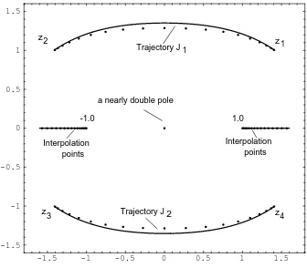
Figure 3.1: 40 poles of the rational interpolantr40,40(f, A80;·)
together with the two arcsJ1, J2 and parts of the
interpolation points inA80.
The interpolation scheme formed by the pointsajn is denoted by A1, and the
inter-polation points ajn will be chosen in such a way that the interpolation schemeA1
has the asymptotic distributionα =α(A1) defined by
dα(x) := √ cxdx
x2 −1√x4−2x2+ 9 =
cxdx q
(x2−1)(x−z
1)· · ·(x−z4)
, x∈I, (3.12)
where the square root in (3.12) is chosen such that the measure is positive, and the constant c= 0.45354. . . has been chosen in such a way that ||α|| = 1. For a given
n∈N the interpolation pointsajn, j = 0, . . . , n, are defined by
α([1, ajn]) = 2j+ 1
2n+ 2 for j = 0, . . . ,[n/2],
α([−∞, ajn]) = 2j−n
2n+ 2 for j = [n/2] + 1, . . . , n.
(3.13)
The symmetric domainD=DA1,f associated with the schemeA1 and the
arcs J1 and J2, which connect the pairs of points {z1, z2} and {z3, z4}, respectively.
The two arcs J1 and J2 are trajectories of a quadratic differential, we have
z2
(z2 −1)(z−z
1)· · ·(z−z4)
dz2 ≤0. (3.14)
-1.5 -1 -0.5 0 0.5 1 1.5
-1.5 -1 -0.5 0 0.5 1 1.5
a nearly double pole Poles of
[40/40] 2
z
3 z
z1
z4 Trajectory C1 2
Trajectory C
Poles of [40/40]
Figure 3.2: 40 poles of the Pad´e approximant [40/40] to the function (3.11) developed at infinity together with the two arcsC1 and C2 that
form the complement of the convergence domain.
In Figure 3.1 the arcsJ1 andJ2 are shown together with the 40 poles of the rational
interpolantr40,40(f,A1;·) =r40,40(f, A80;·) and parts of the 81 interpolation points
of the set A80 = {a0,80, . . . , a80,80} ⊆ I. Of the 40 poles of r40,40 two subsets of 19
elements each cluster to the two arcs J1 and J2 and the two remaining poles form
a nearly double pole close to the origin. These two poles approximate the double pole of f at the origin. From Theorem 3.1 we know that the sequence rnn(f,A1;·),
n = 1,2, . . ., converges to f in capacity in the domain D = C\ (J1 ∪J2). The
convergence of the rational interpolants rnn(f,A1;·), n = 1,2, . . ., is fastest near
the intervalI and becomes slower the nearer one comes to the two arcs J1 and J2.
Example 3.2: The function f is again defined by (3.11), but now the function will be interpolated only at infinity. Thus, an interpolation schemeA2 is used that
is defined by
-1.5 -1 -0.5 0 0.5 1 1.5 -1.5
-1 -0.5 0 0.5 1 1.5
Interpolation points
Interpolation points 2
z
3
z
z1
z4
Poles of r
40,40
Poles of r
40,40
Poles of [40/40] Poles of
[40/40]
Figure 3.3: 40 poles of the Pad´e approximant [40/40] together with 40 poles of the rational interpolant r40,40(f,A1,·) and
two subsets of the 81 interpolation points used for the interpolantr40,40(f,A1;·).
The rational interpolants rnn(f,A2;·) are the Pad´e approximants [n/n] developed
at infinity. Again, the symmetric domain in the sense of Definition 3.2 consists of the Riemann sphere C minus two arcs C1 and C2, but now the two arcs connect
the pairs of branch points{z4, z1}and {z2, z3}, respectively. The two arcs are again
trajectories of a quadratic differential, they satisfy
z2
z4−2z2+ 9dz 2
≤0. (3.16)
The arcs C1 and C2 can be characterized by a principle of minimal capacity (cf.
[St5], Theorem 1.3). In Figure 3.2 the arcsC1 and C2 are shown together with the
40 poles of the Pad´e approximant [40/40]. Again, 19 of these poles cluster at each of the two arcsC1 andC2, and two poles form a nearly double pole close to the origin.
Note that the different choices of interpolation points in the schemesA1 and A2
result in rather different shapes of the convergence domains. This in turn results in different convergence behaviors, which can be seen best in a neighborhood of the origin, where different branches of the functionf are approximated by the sequences
{rnn(f,A1;·)} and {[n/n]}. In Figure 3.3 all 40 poles of the Pad´e approximant
with two subsets of the 81 interpolation points used for the interpolantr40,40(f, A1;·).
The two sets of poles mark the boundary of the area on which different branches of the function f are approximated by the two sequences{rnn(f,A1;·)}and {[n/n]}.
Proof of Theorem 3.1: Important aspects of the proof are practically copies of the proof of the Theorems 1.2 and 1.7 in [St5]. The complete proof is rather complex, and compared with this complexity the changes necessary for Theorem 3.1 are only minor. In any case, a complete reproduction of the full proof would be too long for the present paper. Therefore we will only discuss the main changes and shall not try to give a discription that can be understood independently of [St5].
A core piece of the method used in [St5] is to show that the limit
1
nνQn
∗
−−−−→ ω=ωD,α as n→ ∞ (3.17)
holds true, where Qn is the denominator polynomial of the (linearized) rational interpolant rn = rnn(f,A;·), νQn the counting measure that places unit mass at
each zero ofQn(taking account of multiplicities),−−−−→∗ denotes weak convergence in the space of measures, and ωD,α is the measure defined by
ωD,α:=
Z
ωD,xdα(x) (3.18)
withωD,xthe harmonic measure on∂Drepresenting the pointx∈D. As in Theorem 3.1Ddenotes the symmetric domainDA,f andα =α(A) the asymptotic distribution
of the interpolation schemeA.
The measure ωD,α appeared already in the Green potentialg(α, D;·) introduced in (3.2). The potential can be represented as
Z
As in [St4] and [St5] we have to use a definition of logarithmic potentials, which takes special care of masses near infinity. The potentials are defined by
p(µ;z) :=
The use of the normalization implied by (3.21) is necessary since there may be sequences of potentialsp(µ1;·), p(µ2;·), . . . with measures that contain masses such
thatµ1, µ2, . . . tend to infinity in a rather uncontrolled way; the sequence of measures
In the proofs of the Theorems 1.2 and 1.7 in [St5] two Lemmas 3.1 and 3.2 play a fundamental role. There appears a logarithmic potential p(µ+ν1 +ν2;·) with
ν1, ν2, andµmeasures with certain properties. In the new setting this potential has
to be replaced by a potential of the form p(µ+ν1 +ν2 −2α;·), i.e., the role of
infinity is now played by the measureα. In order to avoid complications one should assume∞ ∈D\supp(A), which always can be achieved, without loss of generality, by transforming the whole problem by a Moebius transform.
An important ingredient in the proof of the Lemmas 3.1 and 3.2 of [St5] and also a major tool in the proof of Theorem 1.8 of [St5] is the reflection function Φ introduced in (2.29) of [St5]. It is an anti-analytic, conformal mapping of neighborhoods of the arcs Jj,j ∈I. The arcs Jj are invariant under this map. The existence of the map is a consequence of the symmetry property (3.3), only that in the new setting this property holds with respect to the Green potential g(α, D;·), and not with respect to the Green function gD(z,∞), as is the case in [St5].
The form of the identities (4.2) and (4.3) in Lemma 4.1 of [St5] reflects interpo-lation at infinity. In case of a general interpointerpo-lation scheme A the identity (4.2) of [St5] has to be replaced by
I
Cζ
kQn(ζ)f(ζ)dζ w2n(ζ)
= 0 for k= 0, . . . , n−1, (3.22)
where C is an integration path separating supp(A) from F = C\D, w2n is the
polynomial introduced in (1.3), andQnis the denominator polynomial of the rational interpolant rn = rnn(f,A;·). The formula (4.3) of [St5] for the interpolation error has to be replaced by
(f−rn)(z) = 1 2πi
1 (QnP)(z)
I
C
(QnP f)(ζ)
w2n(ζ) dζ
ζ−z, P ∈ Pn\ {0}. (3.23)
Note that the orthogonality relation (3.22) is the analogue of relation (2.5), which holds in case of rational interpolation of Markov-, Stieltjes-, or Hamburger functions. As a consequence of (3.22) the integral (4.39) in [St5], which is of central interest in the proof of Theorem 1.7 in [St5], has to be replaced by
I
C(PnQnf)(ζ)
dζw2n(ζ)
. (3.24)
There are more technical details that have to be changed, however all these changes follow rather immediately if one follows the logic that has governed the replacement of the formulas (4.2) and (4.3) in [St5] by the formulas (3.22) and (3.23). The reflection on the arcs Jj, j ∈ I, by the function Φ has to be done in exactly the
4
The Existence of Symmetric Domains
We have seen in the last section that the existence of a symmetric domain is a necessary condition for the validity of the proof of Theorem 3.1. Existence theorems for symmetric domains are known in two situations. These cases are reviewed in the Theorems 4.1 and 4.4, below. The section is closed by a discussion of the difficulties that arise in a proof of a more general existence result.
Let the special interpolation scheme with all interpolation points equal to a fixed pointz ∈Cbe denoted byAz. In this case an asymptotic distribution always exist,
and we have α(Az) = δz. The rational interpolants defined by such a scheme are
the Pad´e approximants [n/n] developed at the point z.
Theorem 4.1: Let the function f have all its singularities in a compact setE ⊆C
with cap(E) = 0, and among the singularities there should be branch points. Let further A =Az with z ∈C\E. Then there exists a symmetric domain D=Dz := Df,Az in the sense of Definition 3.2. The domain is unique up to a set of capacity
zero.
Remarks: (1) The assumption that the function f has to have branch points implies that cap(C\Dz)>0.
(2) It is immediate that a Moebius transform maps a symmetric domain again into a symmetric domain. Hence, without loss of generality we can assume in all proofs thatz =∞ in Theorem 4.1.
Theorem 4.1 is an immediate consequence of the Theorems 1 and 2 in [St1] and the Corollary to Theorem 1 in [St2] in case of the special interpolation schemeA∞. From remark 2 we then know that the theorem holds in general. The next theorem follows also from the Theorems 1 and 2 in [St1].
Theorem 4.2: The symmetric domain D = D∞ of Theorem 4.1 is uniquely determined up to a set of capacity zero by the following two conditions:
(i) ∞ ∈D, and the function f has a single-valued meromorphic continuation in D. (ii)cap(C\D) = inf˜
Dcap(C\D˜), where the infimum extends over all domainsD˜ ⊆C that satisfy condition (i).
We note that in [St1] and [St2] domains of single-valued analytic continuation were considered with respect to analyticity and not with respect to meromorphy as in the Definitions 3.1 and 3.2. However, the difference consists only of a denumerable set of isolated points, and therefore this set is of capacity zero and can be neglected. Further, we note that in [St1] and [St2] the domain D exists uniquely, which is the consequence of a third condition in Theorem 1 of [St1] that has not been applied in Theorem 4.2.
Theorem 4.3: Let the function f have all its singularities in a compact set E ⊆C
with cap(E) = 0, and among the singularities there should be branch points. Let further V ⊆ C \ E be a continuum. Then there exists uniquely up to a set of
capacity zero a domain D=Df,V ⊆C such that
(i) V ⊆D, and f has a single-valued meromorphic continuation in D. (ii)cap(V,C\D) = inf˜
Dcap(V,C\D˜), where the infimum extends over all domains
˜
D⊆C that satisfy condition (i).
In the sequel the complement of the domain Dwill be denoted by F, i.e.,
F :=C\D. (4.1)
We will discuss some notions connected with the condenser (V, F). Since the function
f is assumed to have branch points, we have cap(F) = cap(C\D) > 0. For any
continuumV we have cap(V)>0. Consequently, there exists a condenser potential
pV F, which is defined by the following four properties: (i) In the domainR:=D\V
the potential pV F is harmonic, (ii) it is lower semicontinuous in a neighborhood of
V and upper semicontinuous in a neighborhood of F, (iii) we have pV F(z) = 0 for
whereC is a smooth integration path in the domainRseparating the two setsV and
F, ∂/∂n and ds are the normal derivative and the line element on C, respectively. The condenser capacity then is defined as
cap(V, F) := 1
cV F (4.3)
(cf. [Ba]). There exists a probability measure ωV F on V such that
pV F(z) =g(ωV F, D;z) =
is called the equilibrium distribution of the condenser (V, F). In (4.5) ωD,x denotes the harmonic measure on F representing the point x ∈ D; consequently µV F is a probability measure on F.
The measure ωV,F is fundamental for the second situation, in which we have an existence proof for symmetric domains. For each n ∈ N we can select n + 1
interpolation points ajn ∈F, j = 0, . . . , n, such that
The triangular matrix (ajn)j=0,...,n, n=1,2,... forms an interpolation scheme, which we
denote byA=Af,V. By constructionAf,V has ωV F as asymptotic distribution, i.e., α(Af,V) =ωV F.
Theorem 4.4: Let the function f and the continuum V satisfy the assumptions of Theorem 4.3. Then there exists a symmetric domain D = Df,A in the sense of Definition 3.2 that is associated with the function f and the interpolation scheme A=Af,V, and the domain is identical to the domain Df,V in Theorem 4.3 up to a set of capacity zero.
The Theorems 4.1 and 4.4 are so far the only results about the existence of symmetric domains. The existence of symmetric domains in a more general setting is still an open problem. The present section will be closed by an example, which allows to discuss and illustrate some of the difficulties that have to be dealt with in a more general existence proof.
Example 4.1: Let the functionf be defined as
f(z) := √ 1
z2−1, (4.7)
and let y > 1. An interpolation scheme A1 with only two different interpolation
points is defined by
ajn :=i(−1)jy, j = 0, . . . , n, n= 1,2, . . . (4.8)
If a branch of the functionf is interpolated that is analytic on the continuum (inC)
K = [iy, i∞]∪[−i∞,−iy], then by symmetry consideration it is rather immediate that the symmetry domain in the sense of Definition 3.2 is given by
D =Df,A1 :=C\[−1/1]. (4.9)
If we move the two pointsiyand−iycloser to the origin, say 0< y <1, then the idea of minimal capacity, used in Theorem 4.2 for the characterization of symmetric domains with interpolation at infinity, could suggest that in the new situation the symmetric domain is equal to
D=C\([1,∞]∪[−∞,−1]). (4.10)
but this is not the case. Actually, both domains (4.9) and (4.10) are symmetric in the sense of Definition 3.1, and the set [1,∞]∪[−∞,−1] lies even further away from iy and −iy than [−1,1]. But since it has been assumed that a branch of f
is interpolated that is analytic on the continuum K = [iy, i∞]∪[−i∞,−iy], from the two domains (4.9) and (4.10) only the domain (4.9) is symmetric in the sense of Definition 3.2.
Next, we consider an interpolation scheme A2 with four different interpolation
points. Let two real numbersy1 and y2 be given with y1 >1 large and 0 < y2 <1,
let further N ∈N be large, odd, and define the interpolation points ofA2 by
ajn :=
i(−1)jy
1 if j 6≡0 mod(N)
i(−1)jy
2 if j ≡0 mod(N),
(4.11)
j = 0, . . . , n, n = 0,1,2, . . .. If a branch of f is interpolated that is analytic on
the symmetric domain in the sense of Definition 3.2 associated with f and the interpolation scheme A2.
If, however, we interpolate a branch of the function f that is analytic on the continuumK = [iy1, i∞]∪[−i∞, iy2], then the situation becomes more complicated:
IfN ∈Nis sufficiently large, then there exists no symmetric domain in the sense of
Definition 3.2, but symmetric open sets that are defined analoguously. Their union is of the formC\(C1∪C2), whereC1 is an arc connecting the two points−1 and 1,
and separating the point iy2 from the origin, and C2 is a closed curve surrounding
the point iy2. In the two domains Int(C2) and C\(C1 ∪C2 ∪Int(C2)) different
branches of the function f are approximated by the interpolants.
If on the other hand y2>0 is small andN ∈Nis not too large, then there exists
a symmetric domain in the sense of Definition 3.2 associated with f and A2. The
domain is of the formC\C whereC is an arc connecting the two points −1 and 1
and the arc intersects the y-axis betweeniy2 and iy1.
References
[ArEd] Arms, R.J., and Edrei, A.: The Pad´e table and continued fractions gener-ated by totally positive sequences. In: ‘Mathematical Essays dedicgener-ated to A.J. Macintyre, Ohio Univ. Press, Athens, Ohio, 1970, 1-21.
[Ba] Bagby, T.: On interpolation by rational functions. Duke Math. J., 36 (1969), 95-104.
[BaGM] Baker, G.A., Jr., and Graves-Morris, P.R.: Pad´e Approximants. Encycl. Math. Vol. 59, Cambridge University Press, Cambridge, 1996.
[BSW] Baratchart, L., Saff, E.B., and Wielonsky, F.: Rational interpolation of the exponential function. Can. J. Math., 47 (6) (1995), 1121-47.
[Ca] Cauchy, A.L.: Sur la formule de Lagrange relative ´a l’interpolation. Analyse algebraique, Paris (1821).
[Du] Dumas, S.: Sur le d´evelopement des fonctions elliptiques en fractions con-tinues. Th´esis, Univ. Z¨urich, 1908.
[Go] Gonchar, A.A.: On the speed of rational approximation of some analytic functions. Mat. Sb., 105 (147) (1978), English transl. in: Math USSR Sb., 34 (2) (1978), 131-45.
[GoLo] Gonchar, A.A., and L´opez, G.: On Markov’s Theorem for multipoint Pad´e approximants. Mat. Sb., 105 (147) (1978), English transl. in: Math USSR Sb., 34 (1978), 449-59.
[Gu] Gutknecht, M.H.: The rational interpolation problem revisited. Rocky Mountain J. Math., 21 (1991), 263-80.
[Ja] Jacobi, C.G.I.: Ueber die Darstellung einer Reihe gegebener Werte durch eine gebrochene rationale Funktion. Crelle’s J. Reine u. Angew. Math., 30 (1846), 127-56.
[Kr] Kronecker, L.: Zur Theorie der Elimination einer Variablen aus zwei al-gebraischen Gleichungen. Monatsb. koenigl. Preuss. Akad. Wiss. Berlin., (1881), 535-600.
[La] Landkof, N.S.: Foundations of Modern Potential Theory. Springer - Verlag Berlin 1972.
[Lo1] L´opez, G.: On the convergence of multipoint Pad´e approximants for Stielt-jes type functions. Dokl. Acad. Nauk SSSR, 239 (1978), 793-96.
[Lo2] L´opez, G.: Conditions for the convergence of multipoint Pad´e approximants of Stieltjes type functions. Mat. Sb., 107 (149) (1978), English transl. in: Math USSR Sb., 35 (1978), 363-76.
[Lo3] L´opez, G.: On the asymptotics of the ratio of orthogonal polynomials and the convergence of multipoint Pad´e approximants. Mat. Sb., 128 (170) (1985), English transl. in: Math USSR Sb., 56 (1987).
[Lo4] L´opez, G.: Asymptotics of polynomials orthogonal with respect to varying measures. Constr. Approx., 5 (1989), 199-219.
[LoRa] L´opez, G., and Rakhmanov, E.A.: Rational approximations, orthogonal polynomials and equilibrium distributions. In ‘Orthogonal Polynomials and their Applications’, eds. Alfredo, M. et alii. Lect. Notes Math., 1329, Springer-Verlag, Berlin 1988, 125-57.
[Lu] Lubinsky, D.S.: Divergence of complex rational approximants. Pacific J. Math., 108 (1983), 141-153.
[Me] Meinguet, J.: On the solubility of the Cauchy interpolation problem. In: ‘Approximation Theory’, ed. Talbot, A., Academic Press, London 1970, 535-600.
[Mey] Meyer, B.: On convergence in capacity. Bull. Austral. Math. Soc., 14 (1976), 1-5.
[Nu] Nuttall, J.: The convergence of Pad´e approximants of meromorphic func-tions. J. Math. Anal. Appl., 31 (1970), 129-140.
[Pe] Perron, O.: Kettenbr¨uche, Chelsea Publ. Comp., New York, 1929.
[Ra] Rakhmanov, E.A.: On the convergence of Pad´e approximants in classes of holomorphic functions. Math. USSR Sb., 40 (1980), 149-155.
[St1] Stahl, H.: Extremal domains associated with an analytic function I, II. Complex Variables Theory Appl., 4 (1985), 311-324, 325-338.
[St2] Stahl, H.: The structure of extremal domains associated with an analytic function. Complex Variables Theory Appl., 4 (1985), 339-354.
[St3] Stahl, H.: Orthogonal polynomials with complex-valued weight function I, II. Constructive Approximation 2 (1986), 225-40, 241-51.
[St4] Stahl, H.: On the convergence of generalized Pad´e approximants. Construc-tive Approximation 5 (1989), 221-40.
[St5] Stahl, H.: The convergence of Pad´e approximants to functions with branch points. Submitted to J. Approx. Theory.
[StTo] Stahl, H. and Totik, V.: General Orthogonal Polynomials. Encycl. Math. Vol. 43, Cambridge University Press, Cambridge, 1992.
[Ts] Tsuji, M.: Potential Theory in Modern Function Theory. Maruzen, Tokyo 1959.
[Wa1] Wallin, H.: The convergence of Pad´e approximants and the size of the power series coefficients. Appl. Anal., 4 (1974), 235-51.
[Wa2] Wallin, H.: Potential theory and approximation of analytic functions by rational interpolation. In: ‘Proc. of the Colloquium on Complex Analysis at Joensuu’, Lect. Notes Math., 747, Springer-Verlag, Berlin 1979, 434-50.
[Wal] Walsh, J.L.: Interpolation and Approximation by Rational Functions in the Complex Domain. AMS Colloquium Publ. XX, Providence 1960.
TFH - Berlin /FB 2 Luxemburgerstr. 10 13353 Berlin;
Germany
![Figure 3.2: 40 poles of the Pad´e approximant [40/40] to the function (3.11)developed at infinity together with the two arcs C1 and C2 thatform the complement of the convergence domain.](https://thumb-ap.123doks.com/thumbv2/123dok/940265.906453/13.612.113.461.124.466/figure-approximant-function-developed-innity-thatform-complement-convergence.webp)
![Figure 3.3: 40 poles of the Pad´e approximant [40/40] together with40 poles of the rational interpolant r40,40(f, A1, ·) andtwo subsets of the 81 interpolation points used for theinterpolant r40,40(f, A1; ·).](https://thumb-ap.123doks.com/thumbv2/123dok/940265.906453/14.612.160.486.88.374/figure-approximant-rational-interpolant-subsets-interpolation-points-theinterpolant.webp)
