WORLD OR, IS A TRUNCATED HEAVY TAIL HEAVY OR NOT?
ARIJIT CHAKRABARTY AND GENNADY SAMORODNITSKY Abstract. We address the important question of the extent to which random variables and vectors with truncated power tails retain the char-acteristic features of random variables and vectors with power tails. We define two truncation regimes, soft truncation regime and hard trun-cation regime, and show that, in the soft truntrun-cation regime, truncated power tails behave, in important respects, as if no truncation took place. On the other hand, in the hard truncation regime much of “heavy tailed-ness” is lost. We show how to estimate consistently the tail exponent when the tails are truncated, and suggest statistical tests to decide on whether the truncation is soft or hard. Finally, we apply our methods to two recent data sets arising from computer networks.
1. Introduction
Probability laws with power tails are ubiquitous in applications. A good fit between empirical distribution of various quantities of interest and distri-butions with power tails has been reported in such diverse areas as human travel (Brockmann et al. (2006)), earthquake analysis (Corral (2006)), ani-mal science (Bartumeus et al. (2005)) and even in language (Serrano et al. (2009)). It is also true that in many situations there is a “physical” limit that prevents a quantity of interest from taking an arbitrarily large value. The File Allocation Table (FAT) used on most computer systems allows the largest file size to be 4GB (minus one byte) (Microsoft Knowledge Base Ar-ticle 154997 (2007)); the greatest loss an insurance company is exposed to by a single covered event is limited by its reinsurance contract (see e.g. Mikosch (2009)). Even the number of the atoms in the universe is widely considered to be finite. It is common in practice to combine these two facts together and use a model that features power tails only in a truncated form; such models are often referred to as truncated L´evy flights, see e.g. Scholtz and
1991Mathematics Subject Classification. Primary 62G32, 62G10 Secondary 60E07. Key words and phrases. heavy tails, truncation, regular variation, Central Limit theorem, Hill estimator, consistency.
Research partly supported by the ARO grant W911NF-07-1-0078 at Cornell Univer-sity. Gennady Samorodnitsky’s research was also partly supported by a Villum Kann Rasmussen Visiting Professor Grant at the University of Copenhagen and by Otto Moen-sted foundation grant at Danish Technological University.
1
Contreras (1998), Maruyama and Murakami (2003) or Zaninetti and Ferraro (2008). At the first glance this leads to a situation where the power tails, in a sense, completely disappear. The truncation may change dramatically the behavior of the cumulative sums of observations and it always changes dra-matically the behavior of the cumulative maxima of the observations. Yet it is precisely such patterns of behavior for which a model with power tails is chosen in the first place. This leads one to ask the natural question: to what extent, if any, do phenomena well described by models with truncated power tails retain the characteristic features of power tails?
Answering this question is not straightforward. We start by pointing out that the level of truncation is linked to the amount of observations one has at hand. This can be thought of in different ways. First of all, finiteness of the sample is sometimes taken as the source of the truncation, see e.g. Burrooughs and Tebbens (2001) or Barthelemy et al. (2008). Secondly, both the physical nature of the truncation bound and the available data can be linked to a technological level. This is particularly transparent when one models a phenomenon related to computer or communications systems; see e.g. Jelenkovi´c (1999) or Gomez et al. (2000). We describe this situation as a sequence of models, each one with truncated power tails or, in other words, as a triangular array system, which we now proceed to define formally.
Let F be a probability law on Rd, d ≥ 1, with the following property. There exists a sequence (bn) withbn ↑ ∞ and a non-null Radon measureµ on Rd\ {0}with µ
Rd\Rd}= 0, such that
(1.1) nF b−n1· v
−→µ(·)
vaguely in Rd \ {0}. Here Rd is the compactification of Rd obtained by adding to the latter a ball of infinite radius centered at the origin. The measure µ has necessarily a scaling property: there exists α >0 such that for any Borel set B ∈ Rd and c > 0, µ(cB) = c−αµ(B). We say that the probability law F has regularly varying tails with the tail exponent α
(see Resnick (1987), Hult et al. (2005)), and we view F as the law with non-truncated power tails. When studying the extent to which the central limit theorem behavior is affected by truncation (which is the main point of interest to us in the present paper) we will assume that 0 < α < 2. This restriction on the tail exponent α is precisely the one that guarantees that
F is in the domain of attraction of anα-stable law; see e.g. Rvaˇceva (1962). Such a restriction on the values of the tail exponent will not be necessary in other parts of the paper.
following mechanism:
(1.2) Xnj :=Hj1 kHjk ≤Mn
+ Hj kHjk
(Mn+Rj)1 kHjk> Mn
,
j = 1, . . . , n, n= 1,2, . . .. HereH1, H2, . . . are i.i.d. random vectors in Rd
with the common lawF that has regularly varying tails with a tail exponent
α ∈ (0,2), and R1, R2, . . . are an independent of H1, H2, . . . sequence of
i.i.d. nonnegative random variables. For each n = 1,2, . . . we view the observations Xnj, j = 1, . . . , n as having power tails that are truncated at levelMn.
We need to comment, at this point, on the role of the random variables
R1, R2, . . .. One should view them as possessing light tails, even
exponen-tially decaying tails. In many cases taking these random variables to be equal to zero with probability 1 is appropriate; in other applications expo-nentially fast tapering off of the tails beyond the truncation point has been observed (see e.g. Hong et al. (2008)). The reader will notice that the results of this paper hold whenever the tails of the random variablesR1, R2, . . .are
only light enough, not necessarily exponentially light. We have chosen to formulate our results in this way in order to increase their generality, even though we are thinking of their role in the model (1.2) as representing the exponentially fast decaying tails.
Our approach to addressing the question “to what extent do models with truncated power tails retain the characteristic features of power tails?” lies in studying the effect of the rate of growth of the truncation levelMnon the asymptotic properties of the triangular array defined in (1.2). Specifically, we introduce the following definition. We will say that the tails in the model (1.2) are
(1.3) truncated softly if limn→∞nP kH1k> Mn
= 0,
truncated hard if limn→∞nP kH1k> Mn=∞.
Clearly, an intermediate regime exists as well. Understanding the various aspects of an intermediately truncated model is an interesting theoretical question, that we largely leave aside in this paper, in order to keep its size manageable (see, however, Remark 1 of Section 2). For practical purposes the soft and hard truncation regimes provide the main dichotomy.
is to find out whether the tails in the sample are truncated softly or hard. In Section 4, where we suggest statistical procedures for testing the hypothesis of the soft (correspondingly, hard) truncation regime against the appropriate alternative. In Section 5 we apply the statistical techniques of Section 4 to two recent data sets related to TCP connections in a large computer network. The goal for that section is only to illustrate the statistical tests discussed in Section 4.
We finish this section by pointing out that some of the issues related to models with power tails that have been “tampered with”, have been ad-dressed in the literature. The goals, points of view or the ways in which the tails are modified were different from what is done in the present work. The paper Asmussen and Pihlsgard (2005) discusses an application of dis-tributions with truncated power tails in queuing, and addresses the question whether light tailed approximations or heavy approximations work better in this situation. On the other hand, a maximum likelihood estimation pro-cedure of the tail exponent α in a parametric model of truncated power tails (specifically, the truncated Pareto distribution) is given in Aban et al. (2006). Estimation of the tail exponent in randomly censored power models (where the tails are not so much truncated, as contaminated) is discussed in Beirlant et al. (2007) and Einmahl et al. (2008). Finally, the Hill estimator for censored data is discussed in Beirlant and Guillou (2001). The tech-niques for dealing with censored tails are consistent with the earlier work of Cs¨orgo et al. (1986).
2. A Central Limit Theorem for random vectors with truncated power tails
Consider the triangular array defined in (1.2), where, as we recall, the random vectors H1, H2, . . . have a distribution with regularly varying tails
with a tail exponent α ∈(0,2). This means that these random vectors (or their law F) are in the domain of attraction of some α-stable law ρ on Rd (see Rvaˇceva (1962)). That is, the partial sums Sn(H) = H1 +. . .+Hn,
n= 1,2, . . ., converge in law, after appropriate centering and scaling, to ρ. Defining the sums of thetruncated observations,
Sn:= n
X
j=1
Xnj, n= 1,2, . . . ,
2.1. Soft truncation regime: truncated heavy tails are still heavy.
We start with the situation where the truncation levelMngrows sufficiently fast with the sample size, so that the truncated power tails model (1.2) is in the soft truncation regime. Theorem 2.1 below shows that, in this case, the partial sums of the random vectors with truncated heavy tails converge, when properly centered and scaled, to the same α-stable limit as without truncation.
Let (cn) and (bn) denote, respectively, some centering and scaling se-quences for the non-truncated random vectors (Hj), that is,
(2.1) b−n1Sn(H)−cn=b−n1 n
X
j=1
Hj −cn=⇒ρ
asn→ ∞.
Theorem 2.1. In the soft truncation regime we have (2.2) b−n1Sn−cn=⇒ρ . Proof. By (2.1) it is enough to show that
b−n1
Sn− n
X
j=1 Hj
p −→0.
However, for anyε >0,
P
b−n1
Sn− n
X
j=1 Hj
> ε
≤P
kHjk> Mn for somej= 1, . . . , n
≤nP kH1k> Mn→0,
and the claim follows.
2.2. Hard Truncation regime: truncated heavy tails are no longer heavy. Now we consider the situation where the truncation levelMngrows relatively slowly with the sample size, and that the truncated power tails model (1.2) is in the hard truncation regime. As we will see, in this case the partial sums of the random vectors with truncated heavy tails are no longer asymptoticallyα-stable but, rather, converge in law, after suitable centering and scaling, to a Gaussian limit. Therefore, at least from the point of view of the behavior of partial sums, a model with power tails that have been truncated hard does not behave anymore as a heavy tailed model.
We start with some preliminaries. Recall that, since the limiting lawρin (2.1) is α-stable, the L´evy-Khinchine formula for its characteristic function has the form
(2.3) ρˆ(θ) = exp
ihθ, γi
+
Z
S
Z ∞
0
n
eixhθ,si−1−ixhθ, si1(x≤1)ox−(1+α)dx
Γ(ds)
forθ∈Rd, whereγ ∈Rd, and Γ is a finite measure on the unit sphere inRd,
S :={x∈Rd:kxk= 1}, see Theorem 6.15 in Araujo and Gin´e (1980). The measure Γ is often referred to as spectral measure of the lawρ; see Theorem 2.3.1 in Samorodnitsky and Taqqu (1994).
Theorem 2.2. Assume thatER21<∞, and let
Bn:=
nMn2P(kH1k> Mn)
1/2
, n= 1,2, . . . .
Then in the hard truncation regime we have
(2.4) Bn−1(Sn−ESn) =⇒η ,
where η is a centered Gaussian law on Rd whose covariance matrix has the entries
(2.5) 2
2−α
Z
S
sisjΓ(˜ ds), i, j= 1, . . . , d ,
where Γ(˜ ·) := Γ(·)/Γ(S) is the normalized spectral measure ofρ. We start with a lemma.
Lemma 2.1. For every continuous function f :S −→R, lim n→∞nB −2 n Z S
Z Mn
0
f(s)r2P
kH1k ∈dr, H1
kH1k ∈ds
= α
2−α
Z
S
f(s) ˜Γ(ds).
Proof. Assumption (2.1) means that
(2.6)
PkH1k> r, H1
kH1k ∈ ·
P kH1k> r =⇒Γ(˜ ·)
weakly on S; see e.g. Corollary 6.20 (b) of Araujo and Gin´e (1980). There-fore,
Z
S
Z Mn
0
f(s)r2P
kH1k ∈dr, H1
kH1k
∈ds
=
Z Mn
0
2y
Z
S
f(s)P
kH1k> y, H1
kH1k
∈ds
dy
−Mn2
Z
S
f(s)P
kH1k> Mn,
H1
kH1k
∈ds
∼
Z
S
f(s) ˜Γ(ds)
Z Mn
0
2yP kH1k> y
dy−Mn2P kH1k> Mn
∼
Z
S
f(s) ˜Γ(ds)
2 2−α −1
Mn2P kH1k> Mn
=n−1Bn2
Z
S
f(s) ˜Γ(ds)
asn→ ∞, where the second asymptotic equivalence follows from the
Proof of Theorem 2.2. By the Cram´er-Wold device it suffices to show that for everyθ inRd,
Bn−1 hθ, Sni −Ehθ, Sni
⇒N
0, 2
2−α
Z
S
hθ, si2Γ(˜ ds)
.
To this end we will use the Central Limit Theorem for triangular arrays under the Lindeberg condition; see e.g. Theorem 2.4, page 345 in Gut (2005). We need to prove that
(2.7) lim
n→∞
n B2
n
Var hθ, Xn1i= 2
2−α
Z
S
hθ, si2Γ(˜ ds)
and that for every ε >0, (2.8) n B2 n E
hθ, Xn1i −E hθ, Xn1i
2
1hθ, Xn1i −E hθ, Xn1i
> εBn
→0
asn→ ∞. In order to prove (2.7), we will show that
(2.9) lim
n→∞
n B2
n
E (hθ, Xn1i)2
= 2
2−α
Z
S
hθ, si2˜
Γ(ds)
while
(2.10) lim
n→∞
n1/2 Bn
E hθ, Xn1i
= 0.
The former claim follows easily from Lemma 2.1 and the weak convergence (2.6) by writing
E (hθ, Xn1i)2
=E(hθ, H1i)21 kH1k ≤Mn
+E hθ, H1i
2
kH1k2
(Mn+R1)21 kH1k> Mn
!
∼n−1Bn2 α
2−α
Z
S
hθ, si2˜
Γ(ds)+ 1+o(1)
Mn2E hθ, H1i
2
kH1k2
1 kH1k> Mn
!
∼n−1Bn2 α
2−α
Z
S
hθ, si2˜
Γ(ds) +Mn2P kH1k> Mn
Z
S
hθ, si2˜
Γ(ds)
=n−1Bn2
α
2−α + 1
Z
S
hθ, si2˜
Γ(ds) =n−1Bnα α
2−α
Z
S
hθ, si2˜
Γ(ds).
For (2.10) we write
E hθ, Xn1i
≤ kθk h
E kH1k1(kH1k ≤Mn)
+MnP kH1k> Mn
i
.
Since
MnP kH1k> Mn≪Mn P(kH1k> Mn)1/2 =n−1/2Bn, the claim (2.10) will follow once we check that
(2.11) lim
n→∞n
1/2B−1
We give separate arguments for the cases α≤1 andα >1.
Case 1 (α≤1): LettingC be a positive constant whose value may change from line to line, by the Karamata theorem,
E[kH1k1(kH1k ≤Mn)] ≤ E
h
kH1k3/21(kH1k ≤Mn)
i 2/3
∼ CMn P(kH1k> Mn)
2/3
= Cn−1/2Bn P(kH1k> Mn)1/6 ≪ n−1/2Bn.
Case 2 (1 < α < 2): Here (2.11) follows trivially from the fact that
E[kH1k1(kH1k ≤Mn)] has a finite limit, while Bn≫n1/2 asα <2. We have now proved (2.7). By (2.10), the remaining condition (2.8) will follow once we check that for everyε >0,
n B2
n
Ehθ, Xn1i
2
1 hθ, Xn1i
> εBn
→0.
This is, however, an immediate consequence of the fact that the hard
trun-cation implies thatBn≫Mn asn→ ∞.
Remark 1. We briefly address the behavior of the partial sums of the random vectors with truncated heavy tails in the intermediate regime
(2.12) lim
n→∞nP(kHk> Mn) =δ∈(0,∞).
It turns out that, in this case, one can use the same centering and scaling sequences {cn} and {bn} as in the non-truncated case (2.1) (or in the soft truncation regime (2.2)), but the limit will be different. In fact,
(2.13) b−n1Sn−cn=⇒ρδ,
whereρδ is an infinitely divisible law on Rd, which is obtained by a certain truncation of the jumps of theα-stable lawρ in (2.3). Specifically,
(2.14) ρˆδ(θ) = exp
ihθ, γδi
+
Z
S
Z δ−1/α(α−1Γ(S))1/α
0
n
eixhθ,si−1−ixhθ, si1(x≤1)ox−(1+α)dx
+δΓ(S)−1neiδ−1/α(α−1Γ(S))1/αhθ,si −1o
Γ(ds)
forθ∈Rd, where
γδ=γ−
Z ∞
δ−1/α(α−1Γ(S))1/α
x−α1(x≤1)dx
Z
S
sΓ(ds).
We sketch the argument. Write
(2.15) b−n1Sn−cn=
b−n1
n
X
j=1
Hj1 kHjk ≤Mn
−cn
+b−n1Mn n
X
j=1 Hj kHjk
1 kHjk> Mn
+b−n1
n
X
j=1 Hj kHjk
Rj1 kHjk> Mn
.
It is easy to check that the last term in the right hand side of (2.15) converges to zero in probability. Since (2.12) implies that
(2.16) Mn
bn
→δ−1/α(α−1Γ(S))1/α
asn→ ∞, Theorem 5.9, p. 129, of Araujo and Gin´e (1980) implies that the first term in the right hand side of (2.15) has a weak limit whose character-istic function is given by
exp
ihθ, γδi
+
Z
S
Z δ−1/α(α−1Γ(S))1/α
0
n
eixhθ,si−1−ixhθ, si1(x≤1)ox−(1+α)dx
Γ(ds)
.
Finally, it follows from (2.16) that the second term in the right hand side of (2.15) is asymptotically equivalent to
δ−1/α(α−1Γ(S))1/α n
X
j=1 Hj kHjk
1 kHjk> Mn
,
and, by (2.6) and (2.12), the sum above converges weakly to the law of the Poisson sumPN
j=1Yj, whereY1, Y2, . . . are i.i.d. S-valued random variables
with the common law ˜Γ, andN is an independent of them Poisson random variable with meanδ. Since the weak limits of the first and the second terms in the right hand side of (2.15) are easily seen to be independent, this shows (2.13).
3. Hill estimator for random variables with truncated power tails
Estimating the tail exponent α is one of the main statistical issues one faces when working with data for which a model with power tails is con-templated. This is a difficult statistical problem because one attempts to estimate a parameter governing the tail behavior in an otherwise nonpara-metric model. By necessity, any estimator one uses has to be based on a vanishing fraction of the available data. The situation is even trickier when one tries to estimate the tail exponent in a sample of observations with truncated power tails. This is the task we address in this section.
2 makes it intuitive that estimating the tail exponent α should be easier if the tails are truncated softly, than in the case when the tails are truncated hard. This is, indeed, the case. However, in this section we are interested in finding a procedure that permits consistent estimation of the tail exponent
α regardless of the truncation regime; this is especially important because the truncation regime is never known (see, however, Section 4 below). Fur-thermore, in this section we do not restrict the values of the tails exponent to the interval (0,2). That is,α can take any positive value.
A number of estimators of the tail exponent of distributions with non-truncated power tails have been suggested; a thorough discussion can be found in Chapter 4 of de Haan and Ferreira (2006). One of the best known and widely used estimators is the Hill estimatorintroduced by Hill (1975). Given a sample X1, . . . , Xn. the Hill statistic is defined by
(3.1) hn,k=
1
k
k
X
i=1
log X(i)
X(k),
where X(1) ≥ X(2) ≥ . . . ≥ X(n) are the order statistics from the sample
X1, . . . , Xn, andk= 1, . . . , nis a user-determined parameter, the number of the upper order statistics to use in the estimator. The consistency result for the Hill estimator says that, if X1, . . . , Xn are i.i.d. with regularly varying right tail with exponentα >0, andk=kn→ ∞,kn/n→0 asn→ ∞, then
hn,kn → 1/α in probability as n→ ∞; see e.g. Theorem 3.2.2 in de Haan
and Ferreira (2006).
In spite of the simplicity of the statement of the consistency of the Hill estimator, selecting the number k of the upper order statistics for a given sample with nontruncated power tails remains a daunting problem; see e.g. pp. 192-193 in Embrechts et al. (1997). In the main result of this section, Theorem 3.1 below, we will see that one has to be particularly careful when using the Hill estimator on a sample with truncated power tails. Nonetheless, a consistent estimator can still be obtained.
Notice that the next theorem does not impose any conditions on the random variables R1, R2, . . . in the model (1.2).
Theorem 3.1. Suppose that the number kn of the upper order statistics satisfies
(3.2) nP(H1 > Mn) + 1≪kn≪n . Then hn,kn →1/α in probability asn→ ∞.
Note that Theorem 3.1 says that, in the soft truncation regime, the Hill estimator is consistent under the same assumption, kn/n → 0, as in the nontruncated case.
(2007) shows that the result will follow once we check that, under the con-ditions of the theorem,
(3.3) n
kP
Xn1 b(n/k) ∈ ·
v −→µ(·)
vaguely in (0,∞], where µ is a measure on (0,∞] defined by
µ((x,∞]) =x−α for all x >0,
and
b(u) = inf
x >0 : P(H1 > x)≤u−1 , u >0.
Note that (b(n)) is no longer necessarily a sequence satisfying (2.1). In fact, we will use this notation several times in the sequel to denote other quantile-type functions associated with the random variable H1.
By the hypothesis,
lim n→∞
n
kP(H1 > Mn) = 0
and, hence, b(n/k)≪Mn as n→ ∞. Therefore, for any x >0, for nlarge enough,
P
Xn1 b(n/k) > x
= P H1 > xb(n/k)
∼ k
nx
−α
where the last line follows from the hypothesisk≪n and regular variation
of the tail of H1. This shows (3.3).
Since the truncation level Mn is not known, it is desirable to have a sample-based way of deciding on the number of upper order statistics to use in the Hill estimator. A natural (in view of the condition (3.2)) choice is to usea random number of upper order statistics given by
(3.4) ˆkn=
n
1
n
n
X
j=1
1 Xj > γ max i=1,...,nXi
β
,
where γ and β are user-specified parameters taking values in (0,1) and [·] denotes the integer part. The next two theorems show that this choice of the number of upper order statistics leads to a consistent estimator of the reciprocal of the tail exponent. The parameters β and γ can and should be chosen by the user, and the consistency of the estimator depends neither on their choice nor on, for instance, second order regular variation of H1. In
practice, one should, probably, use some version of the so-called Hill plot (see e.g. Embrechts et al. (1997)), by calculating the value of the estimator for a range of β and γ. We leave this issue for future work.
Here the consistency requires that the tail of the random variable R1 is
sufficiently light, relatively to the truncation level.
Theorem 3.2. In the hard truncation regime assume, additionally, that (3.5) P(H1 > Mn)P(R1 > ǫMn) =o(1/n) for all ǫ >0.
If kˆn is chosen as in (3.4), then hn,kˆn→1/αin probability as n→ ∞.
Proof. We start by showing that, asn−→ ∞,
(3.6) ˆkn
kn P −→1,
where
kn:=
h
nP(H1 > γMn)β
i
.
Clearly, all that needs to be shown is
(3.7)
Pn
j=11(Xj > γMˆn)
nP(H1> γMn) P −→1,
where ˆMn:= max1≤i≤nXi. By (3.5),
(3.8) Mˆn
Mn P −→1.
Further, because of the hard truncation,
(3.9)
Pn
j=11(j:Xj > θ1Mn) nP(H > θ2Mn)
P −→
θ1 θ2
−α
for any 0< θ1<1 andθ2>0.
Fix 0 < ǫ < 1. Choose first 0< η < 1 be such that (1−η)−α < 1 +ǫ. Writing
P
Pn
j=11
Xj > γMˆn
nP(H1> γMn)
>1 +ǫ
≤ P[(1−η)Mn>Mˆn] +P
" Pn
j=11(Xj > γ(1−η)Mn)
nP(H1> γMn)
>1 +ǫ
#
and using (3.8) and (3.9), we see that
P
Pn
j=11
Xj > γMˆn
nP(H1> γMn)
>1 +ǫ
Next we chooseη >0 such thatγ(1 +η)<1 and (1 +η)−α>1−ǫ. Writing
P
Pn
j=11
Xj > γMˆn
nP(H1> γMn)
<1−ǫ
≤ P[(1 +η)Mn<Mˆn] +P
" Pn
j=11(Xj > γ(1 +η)Mn)
nP(H1> γMn)
<1−ǫ
#
,
and appealing, once again, to (3.8) and (3.9), we obtain
P
Pn
j=11
Xj > γMˆn
nP(H1> γMn)
<1−ǫ
−→0,
which establishes (3.7), and, hence, also (3.6). In view of (3.6), it suffices to show that
1 kn ˆ kn X i=1
log X(i)
X(ˆkn)
P −→ 1
α.
Fixǫ >0. We choose 0< η <1/2 so thatα−1log1+1−ηη < 3ǫ, and write
P 1 kn ˆ kn X i=1
log X(i)
X(ˆkn) −
1 α > ǫ ≤ P " 1 kn kn X i=1
log X(i)
X(kn)
− 1 α > ǫ 3 # +P
−logX([kn(1+η)])
X([kn(1−η)]) > ǫ 3 +P " ˆ kn kn −1 ≥η # .
It follows from Theorem 3.1 that
P " 1 kn kn X i=1
log X(i)
X(kn+1) −
1 α > ǫ 3 #
−→0.
Since kn≫nP(H1> Mn), we see that
X([kn(1+η)]) X([kn(1−η)])
P −→
1 +η
1−η
−1/α
.
Therefore, by the choice of η,
P
−logX([kn(1+η)])
X([kn(1−η)]) > ǫ
3
−→0.
Next, we show consistency of the Hill estimator using the random number (3.4) of upper order statistics in the soft truncation regime. Note that no assumption on the tail ofR1 is necessary in this case.
Theorem 3.3. In the soft truncation regime, if ˆkn is chosen as in (3.4), thenhn,ˆkn →1/αin probability as n→ ∞.
Proof. Let ˜h(k, n)
denote the Hill sequence based on the random variables
H1, . . . , Hn, i.e.
˜
h(k, n) := 1
k
k
X
i=1
log H(i)
H(k) ,
where 1 ≤ k ≤ n and H(1) ≥ . . . ≥ H(n) are the order statistics of
H1, . . . , Hn. Let β be as in (3.4). It is well known that the random step
function
˜
h([n1−βt], n) :t≥1
converges in probability in D[1,∞), equipped with the topology of uniform convergence on bounded intervals, to the constant deterministic function
c(t) = 1/αfort≥1; see Resnick (2007), page 89. Since
P˜h([n1−βt], n)6=h([n1−βt], n) for some t≥1≤nP(H > Mn)−→0, it follows that
(3.10) h([n1−βt], n) :t≥1−→P c(t) :t≥1
in D[1,∞) as well. By Proposition 3.21 (page 154) in Resnick (1987) and soft truncation, we known that
Nn:= n
X
j=1
1 Xj > γ max i=1,...,nXi
=⇒N := ∞
X
j=1
1Γ−j1/α> γΓ−11/α,
where (Γj :j≥1) is the sequence of the arrival times of the unit rate Poisson process on (0,∞). Using (3.10) and Theorem 4.4 (page 27) in Billingsley (1968) we conclude that
h([n1−βt], n), Nnβ=⇒
1
α, N
β
inD[1,∞)×Nβ, whereNβ :={1,2β,3β, . . .}. Since the evaluation map from
D[1,∞)×Nβ toRdefined by (x, a)7→x(a) is continuous, an appeal to the
continuous mapping theorem finishes the proof.
4. Testing for soft and hard truncation
been truncated softly or hard? In this section we construct statistical tests for testing each of the two hypothesis against the corresponding alterna-tive. As in Section 3 we restrict ourselves to the case of one-dimensional observations and the tail exponent α can take any positive value.
Suppose that we are given a sample X1, . . . , Xn of one-dimensional ob-servations from the model (1.2). As in Section 3, we do not use here the triangular array notation. Neither the precise value of the tail exponent nor the exact distribution of the random variables (Rn) in (1.2) are assumed to be known. However, we will assume that an upper bound on the tail exponentα is known.
This section is split into three subsections, describing, correspondingly, testing the hypothesis of soft truncation, testing the hypothesis of hard truncation, and testing a slightly stronger version of the latter.
4.1. Testing the hypothesis of soft truncation. We consider the fol-lowing problem of testing a null hypothesis against a simple alternative:
(4.1) H0 : P(|H1|> M)≪n
−1 (soft truncation) Halt: P(|H1|> M)≫n−1 (hard truncation)
.
We assume the tail exponentα satisfies
(4.2) α < A <∞,
i.e. an upper bound on the tail exponent is available. As a test statistic we will use
(4.3) Zn(A) :=
Pn
i=1|Xi|A max1≤i≤n|Xi|A
.
The following proposition describes the asymptotic distribution of Zn(A) under the null hypothesis and under the alternative.
Proposition 4.1. (i) Under the hypothesis H0 of soft truncation, (4.4) Zn(A)⇒ΓA/α1
∞
X
j=1
Γ−A/αj ,
where (Γj, j ≥ 1) are the arrival times of a unit rate Poisson process on (0,∞).
(ii) Assume that ERA1 < ∞. Then under the hypothesis Halt of hard
truncation, Zn(A)−→ ∞P . Proof. For part (i), we define
bn= infx >0 : P(|H1|A> x)≤n−1 , n= 1,2, . . . . Note that, for any x >0,
nP b−n1|X1|A> x
∼nP b−n1|H1|A> x
as n → ∞. It follows from Proposition 3.21 (page 154) in Resnick (1987) that we have the following weak convergence of a sequence of point processes on (0,∞]:
(4.5) Nn:=
n
X
j=1 δb−1
n |X1|A ⇒N :=
∞
X
j=1 δ
Γ−A/α j
as n → ∞. Here δa is a point mass at a, and the weak convergence takes place in the space of Radon point measures on (0,∞] endowed with the topology of vague convergence; see Section 3.4 in Resnick (1987). We would like to use the continuous mapping theorem to deduce (4.4) from (4.5), but a preliminary truncation step is necessary.
Forε >0 we define
Zn(A;ε) :=
Pn
i=1|Xi|A1 bn−1|Xi|A> ε
max1≤i≤n|Xi|A
.
Notice thatZn(A;ε) =h(Nn), where for a Radon point measureη =Pjδrj
on (0,∞],
h(η) = η (ε,∞]
maxjrj
.
It is standard (and easy) to check that h is continuous with probability 1 at the Poisson random measure N in (4.5), so by the continuous mapping theorem,
Zn(A;ε)⇒ΓA/α1 ∞
X
j=1
Γ−A/αj 1 Γ−A/αj > ε
.
Therefore, the convergence (4.4) will follow once we check that for every
δ >0,
(4.6) lim
ε→0lim supn→∞ P Zn(A)−Zn(A;ε)> δ
= 0.
To this end, notice that, for any 0< θ <1 we can selectτ >0 so small that
P max1≤i≤n|Xi|A ≤τ bn
≤θ for alln large enough. Then, for all nlarge enough,
P Zn(A)−Zn(A;ε)> δ≤θ+δ−1E τ−1b−n1 n
X
i=1
|Xi|A1 bn−1|Xi|A≤ε
!
=θ+δ−1τ−1nb−n1E|X1|A1 b−n1|X1|A≤ε
=θ+δ−1τ−1nb−n1E|H1|A1 b−n1|H1|A≤ε
∼θ+δ−1τ−1nb−n1(1−α/A)−1(εbn)P |H1|A> εbn
where the second equality holds because of soft truncation, and the first asymptotic equivalence follows from the Karamata theorem. Since A > α, we obtain (4.6) by first lettingε →0 and then θ→ 0. This completes the proof of part (i).
For part (ii), we start with observing that
(4.7)
Pn
i=1|Xi|A
nMA
nP(|H1|> Mn) ≥
Pn
i=1|Hi|A1 Mn/2≤ |Hi| ≤Mn
nMA
nP(|H1|> Mn)
≥(Mn/2)A
Pn
i=11 Mn/2≤ |Hi| ≤Mn
nMA
nP(|H1|> Mn)
∼2−A(2α−1)
in probability. On the other hand, for some constantc >0, by the assump-tion ERA1 <∞,
max
1≤i≤n|Xi|
A≤c MA
n + max
1≤j≤nR A j
=cMnA+o(1)n
a.s. asn→ ∞. Since the truncation is hard, and A > α, we see that
(4.8) maxi=1,...,n|Xi| A
nMA
nP(|H1|> Mn) →0
a.s. asn→ ∞as well. The claim of part (ii) follows from (4.7) and (4.8).
Based on Proposition 4.1, we suggest the following test for the problem (4.1).
(4.9) rejectH0 at significance level p∈(0,1) if Zn(A)> cp(α/A), withcp(θ) such thatP(Z(θ)> cp(θ)) =p, where for 0< θ <1,
(4.10) Z(θ) = Γ11/θ ∞
X
j=1
Γ−j1/θ.
The random variable Z(θ) does not seem to have one of the standard distributions, and we are not aware of any previous studies of the distribu-tion of Z(θ). The following proposition lists some of the properties of this distribution.
Proposition 4.2. The random variable Z(θ) is an infinitely divisible ran-dom variable. It has a density with respect to the Lebesgue measure, and the Laplace transform
(4.11) Ee−γZ(θ)=
1 +γeγ
Z 1
0
e−γxx−θdx
−1
,
γ > γ0, where γ0 <0 is the number satisfying
1 +γ0eγ0 Z 1
0 e−γ0x
Proof. Forδ >0 let
Wδ = ∞
X
j=1
δ+ Γj
−1/θ
.
Then Wδ is an infinitely divisible random variable with the Laplace trans-form
Ee−γWδ = exp
(
−
Z δ−1/θ
0
1−e−γy
θy−(1+θ)dy
)
for all γ ∈R because the L´evy measure of Wδ has a compact support; see Rosi´nski (1990) and Sato (1999). Since
Z(θ)= 1 +d T1/θWT
whereT is a standard exponential random variable independent of Γj :j≥ 1
, it follows that
(4.12) Ee−γZ(θ)=
Z ∞
0
e−te−γEe−γt1/θWtdt
=e−γ
Z ∞
0
e−texp
−t
Z 1
0
1−e−γx
θx−(1+θ)dx
dt
=e−γ
Z ∞
0
exp
−t
e−γ+γ
Z 1
0
e−γxx−θdx
dt
via integration by parts. Since the exponent under the integral is positive if and only if γ > γ0, we obtain (4.11). Additionally, it follows from (4.12)
that
(4.13) Z(θ)= 1 +d Y(T),
where Y(t), t≥0
is a subordinator satisfying
(4.14) Ee−γY(t)= exp
−t
Z 1
0
1−e−γx
θx−(1+θ)dx
, t≥0,
independent ofT. Since a L´evy process stopped at an independent infinitely divisible random time is, obviously, infinitely divisible, so isZ(θ). Further-more, the characteristic function of Y(t) is integrable of the real line for every t > 0, so each Y(t) has a density, and then the same is true for any mixture of (Y(t)). Therefore,Z(θ) has a density.
❍ ❍
❍ ❍
❍❍
p
θ
0.5 0.6 0.7
.05 4.3 5.8 8.2
.025 5.1 6.9 9.8
.01 6.2 8.4 12.1
Forθcloser to 1, the rate of convergence of the truncated sumPN
j=1Γ
−1/θ j asN → ∞is very slow, and in order to obtain upper bounds on the quantiles of the random variable Z(θ) we used Proposition 4.2 as described below. Such upper bounds lead to conservative versions of the test (4.9). We use the exponential Markov inequality: for 0< r <−γ0,
P(Z(θ)≥z)≤e−rzEerZ =e−rz
1−re−r
Z 1
0
erxx−θdx
−1
,
and estimate the integral from above by
Z 1
0
erxx−θdx≤er/kk
θ−1
1−θ+
1
k
k
X
j=2 erj/k
j−1
k
−θ
,
k >1. Usingr=.05 and k= 107 we computed numbers ˜c
p(θ) satisfying
P Z(θ)≥˜cp(θ)
≤p .
These numbers ˜cp(θ) are reported in the following table.
❍ ❍
❍ ❍
❍❍
p
θ
0.8 0.9 0.95
.05 65.43 73.12 127.37
.025 79.29 86.98 141.23
.01 97.62 105.31 159.56
Since we are only assuming that the tail exponent α has a known upper bound as in (4.2), but the exact value ofα may be unknown, a possible way to obtain a conservative estimate of the critical value cp(α/A) in (4.10) is to choose a number A1 > A and use the statistic Zn(A1) instead of Zn(A) in (4.3). By Proposition 4.1, under the null hypothesis, the test statistic converges weakly toZ(α/A1), which is stochastically smaller thanZ(A/A1),
and we obtain a conservative test by modifying (4.9) as follows:
(4.15) rejectH0 at significance level p∈(0,1) if Zn(A1)> cp(A/A1).
4.2. Testing the hypothesis of hard truncation. In this subsection we consider the following problem of testing a null hypothesis against a simple alternative:
(4.16) H0 : P(|H1|> M)≫n
−1 (hard truncation) Halt: P(|H1|> M)≪n−1 (soft truncation)
We still assume that an upper bound (4.2) on the tail exponent is known. For a test statistic in this case we choose a number γ ∈(0,1) and define
(4.17) Zn(A;γ) =
P[γn]
j=1(−1)jX
hA/2i j
2
Pn
j=[γn]+1|Xj|A .
Here ahbi = |a|bsign(a) for real a, b is the signed power. The asymptotic distribution ofZn(A;γ) under the null hypothesis and under the alternative in (4.16) is described in Proposition 4.3 below. Recall the standard notation ofSα(σ, β, µ) for (the distribution of) an α-stable random variable with the scale σ, skewness β and location µ; see Samorodnitsky and Taqqu (1994). For a symmetricα-stable random variable,β=µ= 0. For a positive strictly
α-stable random variable with 0< α <1, one hasβ = 1 andµ= 0. Finally, for 0< α <2, let
Cα=
(
(Γ(1−α) cos(πα/2))−1 ifα6= 1,
2/π ifα= 1,
Proposition 4.3. (i) Assume thatER12A<∞. Then under the hypothesis
H0 of hard truncation,
(4.18) Zn(A;γ)⇒C1(γ)χ21,
whereC1(γ) = 2γ/(1−γ), andχ21is the standard chi-square random variable
with one degree of freedom.
(ii) Under the hypothesis Halt of soft truncation,
(4.19) Zn(A;γ)⇒C2(A;γ) S12 S2 ,
where
C2(A;γ) =
γ
1−γ Cα/A
C2α/A
A/α
,
andS1 and S2 are independent random variables, such thatS1 is a
symmet-ric 2α/A-stable random variable with unit scale, andS2 is a positive strictly
α/A-stable random variable with unit scale.
Proof. The claim of part (i) will follow from the following two statements.
(4.20) 1
(nMA
nP(|H1|> Mn))1/2
[γn]
X
j=1
(−1)jXjhA/2i ⇒
2Aγ A−α
1/2
N(0,1),
and
(4.21) 1
nMA
nP(|H1|> Mn) n
X
j=[γn]+1
|Xj|A→
A(1−γ)
in probability. We prove (4.21) first, and it is enough to show that
(4.22) 1
nMA
nP(|H1|> Mn)
E
n
X
j=[γn]+1
|Xj|A
→
A(1−γ)
A−α
and
(4.23) 1
nMA
nP(|H1|> Mn)2 Var
n
X
j=[γn]+1
|Xj|A
→0.
Note that by the Karamata theorem,
E
n
X
j=[γn]+1
|Xj|A
∼(1−γ)n E |X1|A
= (1−γ)nhE |H1|A1(|H1| ≤Mn)
+E(Mn+R1)AP(|H1|> Mn)
i
∼(1−γ)n
α A−αM
A
nP(|H1|> Mn) +MnAP(|H1|> Mn)
= nMnAP(|H1|> Mn)
A(1−γ)
A−α ,
proving (4.22). A similar calculation gives us
Var
n
X
j=[γn]+1
|Xj|A
∼(1−γ)nVar |X1|A
≤n E |X1|2A
∼ nMn2AP(|H1|> Mn) 2A
2A−α,
and (4.23) follows because the truncation is hard. Therefore, we have estab-lished (4.21).
In order to prove (4.20), note that the triangular array
˜
Xnj:=HjhA/2i1 |Hj|A/2 ≤MnA/2
+ Hj |Hj|
(MnA/2+RA/j 2)1 |Hj|A/2> MnA/2
,
j = 1, . . . , n, n= 1,2, . . ., satisfies the assumptions of Theorem 2.2 (withα
replaced by 2α/A), and, therefore,
1
nMA
nP(|H1|> Mn)
1/2 n X j=1 ˜
Xnj−E
Xn j=1 ˜ Xnj ⇒ 2A A−α
1/2
N(0,1).
The random variables XjhA/2i
form a somewhat different triangular array, namely
XnjhA/2i=HjhA/2i1 |Hj|A/2 ≤MnA/2
+ Hj
|Hj|(Mn+Rj)
A/21 |Hj|A/2> MA/2
n
j = 1, . . . , n, n = 1,2, . . ., but an inspection of the proof of Theorem 2.2 shows that the argument applies equally well to the latter triangular array, so that
1
nMA
nP(|H1|> Mn)1/2
n
X
j=1
XnjhA/2i−E
n
X
j=1
XnjhA/2i
⇒
2A A−α
1/2
N(0,1).
In particular, (extending the length of the rows of the triangular array) we see that
1 (nMA
nP(|H1|> Mn))1/2
n
X
j=1
XnjhA/2i−
2n
X
j=n+1 XnjhA/2i
⇒
4A A−α
1/2
N(0,1).
Replacing n with [nγ/2], we obtain (4.20) and, hence, finish the proof of part (i).
For part (ii), we define
bn= inf
x >0 : P(|H1|A/2 > x)≤n−1 , n= 1,2, . . . .
Then for some centering sequence (cn) we have
b−n1
n
X
j=1
HjhA/2i−cn
⇒Y
with Y having a S2α/A(σ, β, µ) distribution with σ2α/A = (C2α/A)−1 and someβ, µ; see Feller (1971). Because of the soft truncation, the triangular array XnjhA/2i
satisfies Theorem 2.1, and so
b−n1
n
X
j=1
XnjhA/2i−cn
⇒Y
with the sameY. Extending the rows of the triangular array gives us
b−n1
n
X
j=1
XnjhA/2i−
2n
X
j=n+1 XnjhA/2i
⇒
2
C2α/A
A/(2α)
S1,
where S1 is a symmetric 2α/A-stable random variable with unit scale.
Re-placingn with [nγ/2] we obtain
(4.24)
[γn]
X
j=1
(−1)jXjhA/2i⇒
γ C2α/A
A/(2α)
Next, we also have
b−n2
n
X
j=1
|Hj|A⇒
1
Cα/A
A/α
S2,
where S2 is a positive strictly α/A-stable random variable with unit scale;
see once again Feller (1971). As before, because of the soft truncation, Theorem 2.1 applies, and we obtain
b−n2
n
X
j=1
|Xnj|A⇒
1
Cα/A
A/α
S2.
Replacing nwith (1−γ)n, shows that
(4.25) b−n2
n
X
j=[γn]+1
|Xj|A⇒
1−γ Cα/A
A/α
S2.
Since the numerator and the denominator of the statisticZn(A;γ) in (4.17) are independent, the claim of part (ii) of the proposition follows from (4.24)
and (4.25).
Interestingly, the asymptotic distribution of the test statistic Zn(A;γ), under the null hypothesis, does not depend on the choice of the parameter
A (as long as it an upper bound on the tail exponent α). Furthermore, under the null hypothesis this asymptotic distribution of the test statistic is light-tailed (e.g. some exponential moments are finite). On the other hand, the asymptotic distribution of the test statistic under the alternative is, clearly, heavy tailed, as even the second moment is infinite. Therefore, a reasonable test will reject the null hypothesis in favor of the alternative if the test statistic is too large. That is, we suggest the following test for the problem (4.16).
(4.26) rejectH0 at significance levelp∈(0,1) if Zn(A;γ)> 2γ 1−γcp,
withcp such thatP(χ21> cp) =p.
4.3. Testing a stronger version of the hypothesis of hard trunca-tion. The test statistics Zn(A;γ) we used in the previous subsection for the problem (4.16) has a nondegenerate asymptotic distribution under both the null hypothesis and the alternative. This may restrict the power of the resulting test. In order to obtain a more powerful test we strengthen the null hypothesis. Specifically, in this subsection we consider the following problem of testing a null hypothesis against a simple alternative:
(4.27) H0: n
1−ǫP(|H
1|> M)≫1 Halt: nP(|H1|> M)≪1
,
For this problem one can use the same test statisticZn(A) defined in (4.3) as we used for the problem (4.1) of testing the hypothesis of soft truncation. Proposition 4.1 tells us that this test statistic diverges in probability to in-finity under the hypothesis of hard truncation. The strengthened hypothesis of hard truncation in (4.27) allows us to quantify how fast this divergence takes place. This, in turn, can be used to build a test. The asymptotic distribution of Zn(A) under the hypothesis of soft truncation is described in Proposition 4.1. The next result provides an asymptotic distributional lower bound on the test statistic under the null hypothesis in the problem (4.27). As in the previous subsections, we assume that an upper bound (4.2) on the tail exponent is known.
Proposition 4.4. Assume thatER2A
1 <∞. Then under the strengthened
hypothesis H0 of hard truncation,
(4.28) lim inf
n→∞ P
n−ǫ/2Zn(A)> x
≥e−x2
for everyx >0.
Proof. In the notation of the triangular array (1.2), consider the binomial random variable Nn = Pnj=11 |Hj| > Mn. The strengthened hypothesis of hard truncation implies that P(Nn ≥nǫ) → 1 as n→ ∞. Notice that, on an event of probability increasing to 1,
Zn(A)≥
Pn
j=1(Mn+Rj)A1 |Hj|> Mn
maxj=1,...,n(Mn+Rj)A1 |Hj|> Mn
≥
Pn
j=1RAj1 |Hj|> Mn maxj=1,...,nRAj1 |Hj|> Mn
.
Therefore, for x >0, using the assumption ER21A<∞, we have
lim inf n→∞ P
n−ǫ/2Zn(A)> x
≥lim inf n→∞ P
max j=1,...,Nn
RAj < n−ǫ/2NnER A
1
2 x −1
≥lim inf n→∞ E
"
1− x
2
Nn
Nn
1Nn≥nǫ
#
→e−x2,
as required.
Proposition 4.4 tells us that under the hypothesis H0, n−ǫ/2Zn(A) is, asymptotically, stochastically larger than the square root of the standard exponential random variable (independently of the parameterA). Therefore, we suggest the following test for the problem (4.27).
(4.29)
rejectH0 at significance level p∈(0,1) if Zn(A)≤
log(1−p)
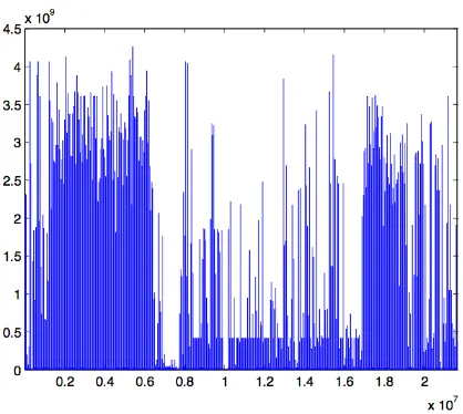
Figure 1. Think Times - the entire data set
5. Think Times and Object Sizes data: soft truncation or hard truncation?
In this section we applied the statistical methods of Section 4 to two data sets. One data set contains “think times”, or delays (in microseconds) between successive request/response exchanges between hosts using a TCP connection. The second data set contains the sizes (in bytes) of objects (files, HTTP responses, email messages, etc.) transferred on TCP connections. Both data sets were acquired by monitoring between 1:30 PM and 2:30 PM on July 24, 2006, the communication links connecting the site of a large commercial enterprize to the Internet. Both data sets exhibit visual evidence of heavy tails, and the Hill estimator confirms that (see below). Our goal is to check if the data sets show statistical evidence of soft or hard truncation of heavy tails. As we will see, in a number of cases we are not able to reject either the hypothesis of soft truncation or that of hard truncation. This is an indication that there is much room for improving the statistical techniques of testing for the type of the truncation of the tails that provides the best approximation to data. We will comment more on that issue at the end of the section.
5.1. Think Times. This data sets contains 2.1×10⁷ observations which are plotted on Figure 1.
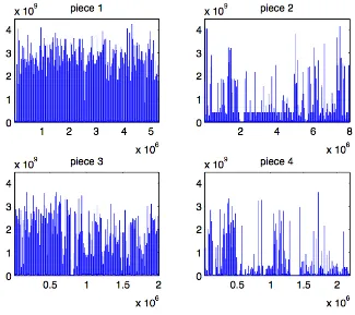
Clearly, the nature of this data set changes over time, and the nature of truncation of heavy tails may potentially change as well. In order to study this effect we have, somewhat arbitrarily, broken the data set into four pieces, with corresponding ranges
0.11×107,0.64×107
;
0.8×107,1.6×107
;
1.7×107,1.9×107
and
1.95×107,2.1×107
Figure 2. Think Times - the different pieces
The structure of the 4 individual pieces appears to be more stable than that of the entire data sets, and we proceed to analyze each piece separately. To do that, we first ran the Hill estimator with random k given in (3.4) on the first half of each of the 4 pieces. The estimation was conducted using β, γ = 0.3,0.4,0.5,0.6,0.7 and conservative upper bounds for α were obtained; these are presented in the following table.
piece A
1 3.02 2 2.30 3 0.85 4 2.24
We then proceeded to use the second halves of each piece of the Think Times data set to test for soft and hard truncations.
Testing the hypothesis of soft truncation. The test statisticZn(A1) of Section 4.1 was computed for various values of A1 larger than A. The results are
A/A1 piece 1 piece 2 piece 3 piece 4
0.5 31.43 5.81 154.05 3.57 0.6 51.59 7.99 205.37 4.72 0.7 77.39 10.74 271.27 6.11 0.8 108.08 14.20 361.74 7.81 0.9 142.78 18.57 491.31 9.91 0.95 161.38 21.16 576.73 11.13
Comparing the resulting values of the test statistic with the corresponding quantiles (or their upper bounds) of Z(A/A1), it is clear that the null
hy-pothesis of soft truncation can be rejected for pieces 1 and 3 at the levels less that 0.01, while for piece 2 the null hypothesis of soft truncation can be rejected at the level 0.025, but not at the level 0.01. For piece 4 we cannot reject the null hypothesis of soft truncation even at the level 0.05. These findings are rather consistent with visual analysis of the pieces of the data set: piece 4 exhibits extremes that do not appear to be seriously truncated (one has to keep in mind that the visual analysis can easily be misleading).
Testing the hypothesis of hard truncation. The test statisticZn(A;γ) of Sec-tion 4.2 was computed for various values of γ. The resulting p-values are reported in the following table.
γ piece 1 piece 2 piece 3 piece 4 0.1 0.85 0.72 0.88 0.33 0.2 0.83 0.98 0.38 0.57 0.3 0.97 0.99 0.79 0.68 0.4 0.94 0.68 0.39 0.43 0.5 0.83 0.63 0.94 0.47 0.6 0.97 0.89 0.83 0.27 0.7 0.91 0.88 0.87 0.40 0.8 0.64 0.85 0.80 0.33 0.9 0.70 0.37 0.85 0.40
The hypothesis of hard truncation cannot be rejected for any of the four pieces. As expected, the p-values for piece 4 are lower than those for the other 3 pieces, but they are still rather high.
Testing a stronger version of the hypothesis of hard truncation. The test statisticsZn(A) of Section 4.3 was computed and the correspondingp-values calculated for various values of ǫ. These are listed in the following table.
ǫ piece 1 piece 2 piece 3 piece 4 0.1 1.00 1.00 1.00 1.00 0.2 1.00 1.00 1.00 1.00 0.3 1.00 1.00 1.00 0.91 0.4 1.00 0.73 1.00 0.45
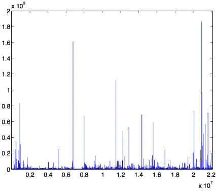
Figure 3. Data on Object Sizes
5.2. Object Sizes. This data set contains 2.2×10⁷ observations. It is plotted in Figure 3. It does not appear that the nature of the observations changes with time, so we applied our statistical tests to the entire data set. After running the Hill estimator with random kand parametersβ and γ as above, on the first half of the data set, we obtained a conservative upper bound on the value of the tail exponent α; this turned out to be A= 1.69. We used the second half of the Object Sizes data set to test for soft and hard truncations.
Testing the hypothesis of soft truncation. We evaluated the test statistic
Zn(A1) of Section 4.1 for a range of values of A1 larger thanA. The results
are reported in the following table.
A/A1 Zn(A1) 0.5 1.75 0.6 2.32 0.7 3.09 0.8 4.10 0.9 5.42 0.95 6.23
Comparing these with the corresponding quantiles (or their upper bounds) ofZ(A/A1), we see that the hypothesis of soft truncation cannot be rejected.
Testing the hypothesis of hard truncation. We evaluated the test statistic
γ p-value 0.1 0.50 0.2 0.36 0.3 0.73 0.4 0.77 0.5 0.95 0.6 0.94 0.7 0.94 0.8 0.97 0.9 0.72
The null hypothesis of hard truncation cannot be rejected.
Testing a stronger version of the hypothesis of hard truncation. We calcu-lated the test statisticsZn(A) of Section 4.3 for various values ofǫ, and the
p-values are given in the following table.
ǫ p-value 0.1 1.00 0.2 0.86 0.3 0.33 0.4 0.08
The strengthened hypothesis of hard truncation becomes suspicious forǫ= 0.4, but overall our statistical tests do not produce clear evidence of the level of truncation for the Object Sizes data set.
Summary The results of this section, especially the lack of conclusion in a number of cases, point to some of the directions for future statistical work with truncated heavy tails.
• More powerful tests are needed, together with estimates of their actual power.
• What sample sizes are necessary for the asymptotic significance lev-els to be applicable?
• The tests of Section 4 depend on tuning parameters A and γ. At present we do not have a clear picture of the role of these parameters, or how to select them in the “optimal” way.
• What is the best way to select the parametersβandγ in the sample-based number of the upper order statistics in (3.4) to use in Hill estimation? Can one combine estimation of the tail index with the testing for a truncation regime in a single procedure?
6. Acknowledgment
References
Aban, I., Meerschaert, M., and Panorska, A. (2006). Parameter estimation for the truncated Pareto distribution. Journal of the American Statistical Association, 101(473):270–277.
Araujo, A. and Gin´e, E. (1980). The Central Limit Theorem for Real and Banach Valued Random Variables. Wiley, New York.
Asmussen, S. and Pihlsgard, M. (2005). Performance analysis with trun-cated heavy-tailed distributions. Methodology and Computing in Applied Probability, 7(4):439–457.
Barthelemy, P., Bertolotti, J., and Wiersma, S. (2008). A L´evy flight for light. Nature, 453:495–498.
Bartumeus, F., da Luz, M., Vishwanathan, G., and Catalan, J. (2005). Animal search strategies: a quantitative random walk analysis. Ecology, 86(11):3078–3087.
Beirlant, J. and Guillou, A. (2001). Pareto index estimation under moderate right censoring. Scandinavian Actuarial Journal, 15(2):111–125.
Beirlant, J., Guillou, A., Dieckx, G., and Fils-Villetard, A. (2007). Esti-mation of the extreme value index and extreme quantiles under random censoring. Extremes, 10(3):151–174.
Billingsley, P. (1968). Convergence of Probability Measures. Wiley, New York.
Brockmann, D., Hufnagel, L., and Geisel, T. (2006). The scaling laws of human travel. Nature, 439:462–465.
Burrooughs, S. and Tebbens, S. (2001). Upper-truncated power laws in natural systems. Pure and Applied Geophysics, 158(4):741–757.
Corral, A. (2006). Universal earthquake-occurence jumps, correlations with time, and anomalous diffusion. Physical Review Letters, 97(17):178501. Cs¨orgo, S., Horv´ath, L., and Mason, D. (1986). What portion of the sample
makes a partial sum asymptotically stable or normal? Probability Theory and Related Fields, 72:1–16.
de Haan, L. and Ferreira, A. (2006). Extreme Value Theory: An Introduc-tion. Springer, New York.
Einmahl, J., Fils-Villetard, A., and Guillou, A. (2008). Statistics of extremes under random censoring. Bernoulli, 14(1):207–227.
Embrechts, P., Kl¨uppelberg, C., and Mikosch, T. (1997).Modelling Extremal Events for Insurance and Finance. Springer-Verlag, Berlin.
Feller, W. (1971). An Introduction to Probability Theory and its Applica-tions, volume 2. Wiley, New York, 2nd edition.
Gomez, C., Selman, B., Crato, N., and Kautz, H. (2000). Heavy–tailed phenomena in satisfiability and constraint satisfaction problems. Journal of Automated Reasoning, 24(1-2):67–100.
Gut, A. (2005). Probability: A Graduate Course. Springer.
Hong, S., Rhee, I., Kim, S., Lee, K., and Chong, S. (2008). Routing perfor-mance analysis of human-driven delay tolerant networks using the trun-cated levy walk model. In Mobility Models ’08: Proceedings of the 1st ACM SIGMOBILE workshop on Mobility models, pages 25–32, New York. ACM.
Hult, H., Lindskog, F., Mikosch, T., and Samorodnitsky, G. (2005). Func-tional large deviations for multivariate regularly varying random walks. Annals of Applied Probability, 15(4):2651–2680.
Jelenkovi´c, P. R. (1999). Network multiplexer with truncated heavy-tailed arrival streams. INFOCOM ’99. Eighteenth Annual Joint Conference of the IEEE Computer and Communications Societies. Proceedings. IEEE, 2:625–632.
Maruyama, Y. and Murakami, J. (2003). Truncated L´evy walk of a nan-ocluster bound weakly to an atomically flat surface: Crossover from su-perdiffusion to normal diffusion. Physical Review B, 67(8):085406. Microsoft Knowledge Base Article 154997 (2007). Description of the FAT32
file system.
Mikosch, T. (2009). Non-Life Insurance Mathematics: An Introduction with the Poisson Process. Springer, Berlin, 2nd edition.
Resnick, S. (1987). Extreme Values, Regular Variation and Point Processes. Springer-Verlag, New York.
Resnick, S. (2007). Heavy-Tail Phenomena : Probabilistic and Statistical Modeling. Springer, New York.
Rosi´nski, J. (1990). On series representation of infinitely divisible random vectors. The Annals of Probability, 18:405–430.
Rvaˇceva, E. (1962). On domains of attraction of multi-dimensional distri-butions. Selected Translations in Mathematical Statistics and Probability, 2:183–205. Publisher: IMS-AMS.
Samorodnitsky, G. and Taqqu, M. (1994). Stable Non-Gaussian Random Processes. Chapman and Hall, New York.
Sato, K. (1999). L´evy Processes and Infinitely Divisible Distributions. Cam-bridge University Press.
Scholtz, C. and Contreras, J. (1998). Mechanics of continental rift architec-ture. Geology, 26(11):967–970.
Serrano, M., Flammini, A., and Menczer, F. (2009). Beyond Zipf’s law: Modeling the structure of human language. Technical Report.
Zaninetti, L. and Ferraro, M. (2008). On the truncated Pareto distribution with applications. Central European Journal of Physics, 6(1):1–6.
School of Operations Research and Information Engineering, Cornell Uni-versity, Ithaca, NY 14853, U.S.A.
E-mail address: [email protected]
School of Operations Research and Information Engineering, Cornell Uni-versity, Ithaca, NY 14853, U.S.A.