Full Terms & Conditions of access and use can be found at
http://www.tandfonline.com/action/journalInformation?journalCode=ubes20
Download by: [Universitas Maritim Raja Ali Haji], [UNIVERSITAS MARITIM RAJA ALI HAJI
TANJUNGPINANG, KEPULAUAN RIAU] Date: 11 January 2016, At: 20:35
Journal of Business & Economic Statistics
ISSN: 0735-0015 (Print) 1537-2707 (Online) Journal homepage: http://www.tandfonline.com/loi/ubes20
Heteroscedasticity Robust Panel Unit Root Tests
Joakim Westerlund
To cite this article: Joakim Westerlund (2014) Heteroscedasticity Robust Panel Unit Root Tests, Journal of Business & Economic Statistics, 32:1, 112-135, DOI: 10.1080/07350015.2013.857612 To link to this article: http://dx.doi.org/10.1080/07350015.2013.857612
View supplementary material
Accepted author version posted online: 13 Nov 2013.
Submit your article to this journal
Article views: 485
View related articles
View Crossmark data
Heteroscedasticity Robust Panel Unit Root Tests
Joakim W
ESTERLUNDFaculty of Business and Law, School of Accounting, Economics and Finance, Deakin University,
Melbourne Burwood Campus, 221 Burwood Highway, VIC 3125, Australia ([email protected])
This article proposes new unit root tests for panels where the errors may be not only serial and/or cross-correlated, but also unconditionally heteroscedastic. Despite their generality, the test statistics are shown to be very simple to implement, requiring only minimal corrections and still the limiting distributions under the null hypothesis are completely free from nuisance parameters. Monte Carlo evidence is also provided to suggest that the new tests perform well in small samples, also when compared to some of the existing tests. Supplementary materials for this article are available online.
KEY WORDS: Common factors; Cross-section dependence; GARCH; Panel data; Unconditional heteroscedasticity.
1. INTRODUCTION
Researchers are by now well aware of the potential hazards involved when using augmented Dickey–Fuller (ADF)-type unit root tests in the presence of unattended structural breaks in the deterministic trend. But breaks in the trend are not the only way in which structural instability may arise. Take, for example, the financial literature concerned with the testing of the efficient market hypothesis, requiring that stock returns are stationary, in which case violations of the otherwise so common homoscedas-ticity assumption is more of a rule rather than the exception. In
fact, asPoon and Granger (2003, p. 481) stated in their review
of this literature.
There are several salient features about financial time series and financial market volatility that are now well documented. These include fat tail distributions of risky asset returns, volatil-ity clustering, asymmetry and mean reversion, and comovements of volatilities across assets and financial markets. More recent research finds correlation among volatility is stronger than that among returns and both tend to increase during bear markets and financial crises.
Time-varying volatility is therefore an important source of structural instability. However, as the citation makes clear there is not only the time variation in the volatility of individual stock returns, but also a great deal of similarity in the volatility of dif-ferent assets and markets, a finding that has been confirmed by
numerous studies (see, e.g.,McMillan and Ruiz 2009). When it
comes to unit root testing, while the latter is typically ignored, the most common way to accommodate the former is to assume that the time variation is in the conditionally variance only (see
Seo 1999), which is of course not very realistic. Indeed, Pa-gan and Schwert (1990),Loretan and Phillips (1994),Watson (1999), andBusetti and Taylor (2003), to mention a few, all pro-vided strong evidence against the unconditional
homoscedastic-A previous version of this article was presented at a workshop at Deakin Uni-versity. The author would like to thank seminar participants, and in particular Christoph Hanck, Rolf Larsson, Paresh Narayan, Stephan Smeekes, Jean-Pierre Urbain, Shakeeb Khan (the Editor), an Associate Editor, and two anonymous referees for many valuable comments and suggestions. Financial support From the Jan Wallander and Tom Hedelius Foundation Under research grant number P2009–0189:1 is gratefully acknowledged.
ity assumption for most financial variables, including exchange rates, interest rates, and stock returns.
Of course, unconditional heteroscedasticity is not only a common feature of financial data, but can be found also in
most macroeconomic variables. For example, Kim and
Nel-son (1999),McConnell and Perez Quiros (2000), andKoop and Potter (2000)all showed how the volatility of U.S. gross
domes-tic product (GDP) has declined since the early 1980s.Busetti
and Taylor (2003) considered 16 series of industrial produc-tion and 17 series of inflaproduc-tion. Consistent with the evidence for GDP, most series are found to exhibit a significant decline in variability around the early 1980s. Similar results were reported byCavaliere and Taylor (2009a). Chauvet and Potter (2001) re-ported decreased volatility also in consumption, income, and in aggregate employment, the latter finding is confirmed by results ofWarnock and Warnock (2000). Sensier and van Dijk (2004) considered no less than 214 monthly macroeconomic time se-ries. According to their results, around 80% of the series were subject to a significant break in volatility. The evidence also suggests that there is a great deal of similarity in the volatility within groups of series, such as industries, sectors, and real and nominal variables. Hence, again, the unconditional variance is not only time varying, but also co-moving.
The current article can be seen as a response to the above observations. The purpose is to devise a panel-based test proce-dure that is flexible enough to accommodate not only the “usual suspects” of serial and cross-correlation, but also general (un-conditional) heteroscedasticity. The tests should also be simple. In particular, they should not suffer from the same computa-tional drawback as many of the existing time series tests, which typically involve some kind of resampling and/or
nonparamet-ric estimation (seeBeare 2008;Cavaliere and Taylor 2009b).
The way we accomplish this is by exploiting the information contained in the similarity of both the variance and level of the cross-sectional units, a possibility that has not received any attention in the previous literature. In fact, except for the
re-cent study ofDemetrescu and Hanck (2011), this is the only
© 2014American Statistical Association Journal of Business & Economic Statistics
January 2014, Vol. 32, No. 1 DOI:10.1080/07350015.2013.857612
112
panel investigation that we are aware of to address the issue of heteroscedasticity.
Two tests based on the new idea are proposed. One is designed to test for a unit root in a single time series, while the other is designed to test for a unit root in a panel of multiple time series. Both test statistics are very convenient in that no prior knowledge regarding the structure of the heteroscedas-ticity is needed, and still the implementation is extremely simple, requiring only minimal corrections. The asymptotic analysis reveals that while the test statistics have asymptotic distributions that are free of nuisance parameters under the unit root null, this is not the case under the local alternative, in which power generally depends on both the heteroscedasticity and the cross-correlation. Results from a small Monte Carlo study show that the asymptotic results are borne out well in small samples. In fact, the tests have excellent small-sample properties, even when compared to the competition.
The rest of the article is organized as follows. Section 2
introduces the model, while Section3presents the test statistics
and their asymptotic distributions, which are evaluated in small
samples in Section4. Section5concludes.
2. MODEL AND ASSUMPTIONS
Consider the panel data variableyi,t, wheret =1, . . . , T and
i=1, . . . , N index the time series and cross-sectional units, respectively. The data-generating process (DGP) of this variable is given by
yi,t =αi+ui,t, (1)
ui,t =ρiui,t−1+vi,t, (2)
withvi,tfollowing a stationary autoregressive process of known
order pi<∞ with possibly cross-section dependent and/or
groupwise heteroscedastic errors. In particular, it is assumed
thatvi,tadmits to the following general dynamic common
fac-tor model:
φi(L)vi,t =ei,t (3)
ei,t =′iFt+ǫi,t, (4)
ǫi,t =σm,tεi,t, (5)
whereφi(L)=1−
pi
k=1φkiLk is a polynomial in the lag
op-eratorL,Ft is anr-dimensional vector of common factors, and
m=1, . . . , M+1 indexesM+1 distinct variance groups. As
withpi, initially we will assume thatr (the number of
com-mon factors) andM(the number of variance groups) are known;
some possibilities for how to relax these assumptions in practice
will be discussed in Section3.3. In the assumptions that follow
⌊x⌋signifies the integer part ofxand||A|| =√tr(A′A) is the
Frobenius (Euclidean) norm of the matrixA.
Assumption 1.
(a) εi,tis independent and identically distributed (iid) across
bothiandt withE(εi,t)=0,E(ε2i,t)=1 andE(ε
4
i,t)<
∞;
(b) Ftis iid acrosstwithE(Ft)=0,E(FtFt′)= t >0 and
E(||Ft||4)<∞;
(c) εi,tandFsare mutually independent for alli,t,ands;
(d) ||i||<∞ for all i and
N
i=1i′i/N → >0 as
N → ∞;
(e) φi(L) have all its roots outside the unit circle;
(f) E(ui,s)<∞for alliands= −pi, . . . ,0.
Consider σm,t2 . It is assumed that the cross-section can be
divided into M cross-section homoscedastic groups with the
mth group containing the unitsi=Nm−1+1, . . . , Nm, where
N0=1 andNM+1=N. That is, the heteroscedasticity across
the cross-section is made up ofMdiscrete jumps between
oth-erwise homoscedastic groups. As a matter of notation, in what
follows, if a variable,xm,i say, depends on bothmandi, since
the latter index runs across groups, the dependence onmwill
be suppressed, that is,xm,iwill be written asxi. Note also that
while the sequential group structure assumed here, in which
units i=Nm−1+1, . . . , Nm are arbitrarily assigned to group
m, is without loss of generality. In fact, as we demonstrate in
Section3.3, in applications it is actually quite useful to think of
the cross-section as being ordered.
Assumption 2.
(a) Nm−Nm−1≥qN and Nm= ⌊λmN⌋, where q >0,
λ0< λ1 <· · ·< λM < λM+1,λ0=0 andλM+1=1;
(b) σ2
m,⌊sT⌋→σm2(s)>0 and ⌊sT⌋→ (s)>0 as T →
∞, where σ2
m(s) and (s) are bounded and
square-integrable with a finite number of points of discontinuity;
(c) N
i=1σi,2⌊sT⌋i′i/N →(s)>0 asN, T → ∞.
The parameter of interest,ρi, is assumed to satisfy
Assump-tion 3.
Assumption 3.
ρi =exp
ci NκT
,
whereκ ≥0, andciis iid acrossiwithE(ci)=μcand var(ci)=
σ2
c <∞.ciis independent ofεj,t andFsfor alli,j,t,ands.
Hence, ifci =0, thenρi =1, and thereforeyi,t is unit root
nonstationary, whereas if ci <0 (ci >0), then ρi approaches
one from below (above) and therefore yi,t is “locally”
sta-tionary (explosive) (in the mean). The relevant null
hypothe-sis here is given byH0:c1= · · · =cN =0, which equivalent
to H0:μc=σc2=0. Similarly, the alternative hypothesis of
H1:ci =0 for at least someican be written equivalently asH1:
μc =0 and/orσc2 >0. Assumption 3 therefore greatly reduces
the dimensionality of the testing problem (fromNto only two).
The “closeness” of the local alternative to the null is determined
byκ. The most “distant” alternative is obtained by settingκ =0,
in which caseρi=exp(ci/T) does not depend onN. This is the
typical time series parameterization, which we will be working under when studying the local asymptotic power of our time
se-ries statistic (see Section3.1). Asκincreases, we get closer to the
null, which means that deviations (ci =0) will be more difficult
to detect. The panel statistic that we will consider has
nonnegli-gible local power forκ=1/2 (see Section3.2) and is therefore
able to pick up smaller deviations than the time series statistic.
Remarks.
1. The variance ofǫi,t is a key in our approach. The
assump-tion of “group-wise heteroscedasticity” in the cross-secassump-tion
not only seems like a reasonable scenario in many
applica-tions (see Section3.3for a discussion), but is also one of the
strengths of the approach, as it allows for consistent
estima-tion of the group-specific variances (see Secestima-tion3.1). This is
facilitated by Assumption 2(a), which states that the groups
increase proportionally withN. In this regard, it is quite
ob-vious that while in theory q (the proportion) can be made
arbitrarily small, in applications the value ofqis not
irrele-vant, as larger groups are expected to increase the precision
of the estimated group-specific variances. In Section4, we
discuss the importance ofq in small samples (see also the
supplement for this article).
2. While the heteroscedasticity across the cross-section needs to have the groupwise structure, the heteroscedasticity across time is essentially unrestricted. In the derivations, we assume
thatσ2
m,tand tare nonrandom, which allows for a wide class
of deterministic variance models, including models with
breaks and linear trends. However, provided that σ2
m,t, t,
εi,t, andFtare independent withE(σm,t2 )>0 andE( t)>0,
σ2
m,t and t can also be random. Conditional
heteroscedas-ticity, including generalized autoregressive conditional het-eroscedasticity (GARCH), is permitted too, as heteroscedas-ticity of this form does not affect the asymptotic results.
3. The assumption in Equation (4) is quite common (see, e.g.,
Pesaran 2007; Pesaran, Smith, and Yamagata 2009), and
ensures that the serially uncorrelated error ei,t has a strict
common factor structure. This is more restrictive than the
approximate factor model considered byBai and Ng (2010),
where the idiosyncratic error is allowed to be “mildly” cross-correlated, but is necessary for the proofs. Except for this, however, the above model is actually quite general when it comes to the allowable serial and cross-sectional
dependen-cies. Note in particular how the error in Equation (2) admits
to a general dynamic factor structure of potentially infinite order.
4. The assumption that the mean and variance ofci are equal
acrossiis not necessary and can be relaxed as long as the
cross-sectional averages ofE(ci) and var(ci) have limits such
as μc and σc2, respectively. The assumption that ci is
in-dependent of εj,t and Fs can also be relaxed somewhat.
In particular, note that since under the null of a unit root
c1= · · · =cN =0, correlation between ci, andεj,t and/or
Fsis only an issue under the alternative hypothesis, and then
it can be shown that in the typical panel parameterization of
ρiwithκ=1/2, the effect of correlation betweenciandεj,t
is negligible, although otherwise this is not necessarily so. Unfortunately, such a correlation greatly complicates both the derivation and interpretation of the results, and we there-fore follow the usual practice in the literature and assume that Assumption 3 holds.
3. TEST PROCEDURES
3.1 A Time Series Test
The time series test statistic that we consider, henceforth
denoted by τi, is very simple and can be seen as a version
of the Lagrange multiplier (LM) test statistic for a unit root (see Remark 4). The implementation consists of four steps:
1. Obtain Rˆi,t as the ordinary least-squares (OLS) residual
from a regression ofyi,tonto (yi,t−1, . . . , yi,t−pi).
2. Obtain ˆFt and ˆi by applying the principal components
method toRˆi,t. Compute ˆǫi,t=Rˆi,t−ˆ′iFˆt.1
3. Compute wˆm,t =1/σˆm,t, where σˆm,t2 =
Nm
i=Nm−1+1ǫˆ
2
i,t/
(Nm−Nm−1).
4. Compute
τi =
T
t=pi+2 ˆ
Rwi,tRˆwi,t−1
2
T
t=pi+2Rˆ
2
wi,t−1
,
where i=Nm−1+1, . . . , Nm, Rˆwi,t=wˆm,tǫˆi,t and
ˆ
Rwi,t=tk=pi+2Rˆwi,k. Remarks.
5. τican be seen as a version of the true LM test statistic (based
on known parameters) for testing H0:ci =0, which is
given by (T
t=pi+2w
2
m,tRi,tRi,t−1)2/Tt=pi+2w
2
m,tR
2
i,t−1,
where wm,t=1/σm,t, Ri,t=φi(L)yi,t and Ri,t =
t
k=pi+2Ri,k.
2Unfortunately, the asymptotic distribution
of this test statistic depends on σm(r) and (r), which
means that critical values can only be obtained for a
par-ticular choice of (σm(r), (r)).3 The use of accumulated
weighted first differences (as when replacingwm,tRi,t−1with
t
s=pi+2wm,sRi,s) eliminates this dependence.
6. The formula forτireveals some interesting similarities with
results obtained previously in the literature. In particular,
note howτi is basically the squared, weighted, and
“defac-tored” equivalent of the conventional ADF test. It can also be
regarded as a generalization of the LM test developed byAhn
(1993), and Schmidt and Phillips (1992), who considered the problem of testing for a unit root in a pure time series setting
with homoscedastic errors. The way thatRˆwi,tis
accumu-lated up to levels is very similar to the approach ofBai and
Ng (2004). But while in that article the accumulation is just an artifact of their proposed correction for cross-section de-pendence, here it is used as a means to recursively weight the observations, and ultimately to remove the effect of the
heteroscedasticity (seeBeare 2008, for a similar approach).
7. As is well known, under certain conditions (such as normal-ity), the LM test statistic possesses some optimality proper-ties. While the test statistic considered here is not the true LM statistic, it is similar and is therefore expected to inherit some of these properties. Apart from the resemblance with the true LM statistic, the use of a squared test statistic has the advantage that it does not rule out the possibility of
explo-sive units (ci >0), which seems like a relevant scenario in
many applications, especially in financial economics, where data can exhibit explosive behavior. Explosive behavior is
1Becausep
iis not restricted to be equal across the cross-section, the panel data
variable ˆǫi,t will in general be unbalanced. Therefore, to simplify this step of
the implementation, one may apply the principal components method to the balanced panel comprising the lastT−max{p1, . . . , pN} −1 observations.
2A formal derivation is available upon request.
3Another problem with the true LM test statistic is that the feasible version
is based on using weighted OLS (WLS) to estimate the first-step regression. However, since the weightwm,tis not known, this calls for the use of iterated
WLS.
also more likely ifNis large, which obviously increases the probability of extreme events regardless of the application considered. This is particularly relevant when constructing
pooled panel test statistics (see Section3.2), in which case
positive and negative values ofcimay otherwise cancel out,
causing low power.
8. τi can be modified to incorporate information regarding the
direction of the alternative. Suppose, for example, that one
would like to testH0:ci =0 versusH1:ci <0. A very
sim-ple approach would be to first testH0versusH1. IfH0is
ac-cepted, then we conclude thatyi,tunit root nonstationary and
proceed no further, whereas ifH0is rejected, then the testing
continues by checking the sign of T
t=pi+2Rˆwi,tRˆwi,t−1. Only if the sign is negative do we conclude that the evidence is in favor of stationarity and not of explosiveness. Of course, because of the data snooping, this test would not be correctly sized. A more appropriate testing approach involves
replac-ingτiwith 1(Tt=pi+2Rˆwi,tRˆwi,t−1/T <0)τi, where 1(A)
is the indicator function for the eventA. The asymptotic null
distribution of the resulting joint test statistic can be worked
out by using the results ofAbadir and Distaso (2007).
9. In regression analysis with heteroscedastic errors it is
com-mon practice to use ˆǫi,t2 to estimateσm,t2 . However, asLopez
(2001)pointed out, while unbiased, because of its
asymmet-ric distribution, ˆǫi,t2 is a very imprecise estimator ofσm,t2 .
ˆ
σ2
t,muses more information and is therefore expected to
per-form much better. Beare (2008) used a similar recursive
weighting scheme as the one considered here, but where
σ2
m,tis estimated in a nonparametric fashion, which not only
leads to a very low rate of consistency but also complicates implementation.
The asymptotic distribution ofτi is given in the following
theorem.
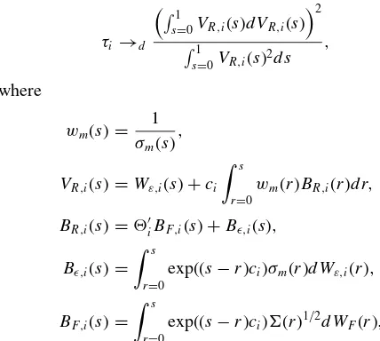
Theorem 1. Under the conditions laid out in Section2, given
κ=0, asN, T → ∞
τi →d
1
s=0VR,i(s)dVR,i(s)
2
1
s=0VR,i(s)
2ds ,
where
wm(s)=
1
σm(s)
,
VR,i(s)=Wε,i(s)+ci
s
r=0
wm(r)BR,i(r)dr,
BR,i(s)=′iBF,i(s)+Bǫ,i(s),
Bǫ,i(s)=
s r=0
exp((s−r)ci)σm(r)dWε,i(r),
BF,i(s)=
s r=0
exp((s−r)ci) (r)1/2dWF(r),
with→d signifying convergence in distribution,i=Nm−1+
1, . . . , Nm, andWε,i(s) andWF(s) being two independent
stan-dard Brownian motions.
To appreciate fully the implication of Theorem 1, note
that sinceVR,i(s) satisfies the differential equationdVR,i(s)=
dWε,i(s)+ciwm(s)BR,i(s)ds, the numerator of the asymptotic
test distribution can be expanded as
1
s=0
VR,i(s)dVR,i(s)=ci
1
s=0
VR,i(s)wm(s)BR,i(s)ds
+
1
s=0
VR,i(s)dWε,i(s).
This illustrates how the presence ofcihas two effects. The first
is to shift the mean of the test statistic and is captured by the first term on the right-hand side, whereas the second is to affect
the variance and is captured byVR,i(s) (which depends onci).
It also illustrates how the local asymptotic power depends on both the heteroscedasticity and the cross-section dependence, as
captured byσ2
m(s) and′iBF,i(s), respectively. Whether this
de-pendence implies higher local power in comparison to the case with homoscedastic errors is not possible to determine unless
a particular choice ofσ2
m(s) and′iBF,i(s) is made. However,
we see that ifσ2
m(s)=σm2andi =0, then the dependence on
these nuisance parameters disappears. We also see that
when-everσm2(s) is not constant and/ori =0, then this is no longer
the case (ifci =0). Note in particular that even ifσm2(s)=σ
2
m,
unless i =0, the dependence on σm2 will not disappear. In
Section 3.2, we elaborate on the power implications of the
heteroscedasticity.
Under the unit root hypothesis that ci =0, dVR,i(s)=
dWε,i(s), and henceVR,i(s)=Wε,i(s), which in turn implies
τi→d
1
s=0Wε,i(s)dWε,i(s)
2
1
s=0Wε,i(s) 2ds
as N, T → ∞. Hence, the asymptotic null distribution of τi
does not depend on σm(s) or ′iBF,i(s). It is therefore
com-pletely free of nuisance parameters. In fact, closer inspection
reveals that the asymptotic distribution ofτi is nothing but the
squared ADF test distribution, which has been studied before
by, for example,Ahn (1993), who also tabulated critical values
(Table 1).
Table 1. Size at the 5% level
N T Case τ τIV SˆN T τi τIV,i
φ1=0
10 100 1 7.0 0.8 3.0 5.3 1.3 20 400 1 5.6 0.1 3.9 5.1 0.4 10 100 2 7.7 1.4 2.7 5.6 2.2 20 400 2 5.6 0.3 3.7 5.2 0.8 10 100 3 8.0 1.5 3.0 5.6 2.3 20 400 3 5.6 0.3 3.8 5.2 0.8
φ1=0.5
10 100 1 8.4 0.0 3.0 5.0 0.3 20 400 1 5.9 0.0 3.6 5.0 0.1 10 100 2 9.3 0.2 3.1 5.5 0.6 20 400 2 6.3 0.0 4.0 5.2 0.2 10 100 3 9.5 0.2 3.1 5.5 0.7 20 400 3 6.4 0.0 4.1 5.2 0.2
NOTES: Variance cases 1–3 refer to homogeneity, a discrete break, and a smooth transition break, respectively.φ1refers to the first-order autoregressive serial correlation coefficient
in the errors.
Remarks.
10. The fact that the asymptotic null distribution ofτiis free of
nuisance parameters is a great operational advantage that is not shared by many other tests. Consider, for example,
the (adaptive) test statistic analyzed by Boswijk (2005),
which allows for heteroscedasticity of the type considered
here (but no cross-section dependence). However, unlikeτi,
the asymptotic distribution of this test statistic depends on
σ2
m(r), which is of course never known in practice.
Simi-larly, while the unit root tests ofPesaran (2007)andPesaran,
Smith, and Yamagata (2009) do allow for cross-section dependence in the form of common factors (but no het-eroscedasticity), their asymptotic null distributions depend
onBF,i(s), whose dimension is generally unknown, which
greatly complicates the implementation. In fact, the only test statistic that we are aware of that comes close to ours in terms of generality and still having a completely nui-sance parameter free null distribution is the Cauchy-based
t-statistic ofDemetrescu and Hanck (2011).
11. The new test statistic can be applied under very general con-ditions when it comes to the dynamics and heteroscedas-ticity of the errors. However, it cannot handle models with a unit-specific trend that needs to be estimated. The reason is that while the effect of the estimation of the intercept is negligible, this is not the case with the trend, whose
estimation introduces a dependence onσm2(s). One way to
circumvent this problem is to use bootstrap techniques (see,
e.g.,Cavaliere and Taylor 2009b). However, this does not
fit well with the simple and parametric flavor of our ap-proach. A feasible alternative in cases with trending data is to assume a common trend slope, which can then be removed by using data that have been demeaned with re-spect to the overall sample mean. That is, instead of using
yi,twhen constructingRˆwi,tone usesyi,t−y, where
y=N
j=1
T
k=pi+2yj,k/N T. The asymptotic
distribu-tion reported in Theorem 1 is unaffected by this.4 Some
limited heterogeneity can also be permitted in this way by
assuming that the trend slope,βisay, is “local-to-constant.”
Specifically, supposed that instead of (1), we have
yi,t=αi+βit+ui,t,
where βi =β+bi/Tγ,γ >1 andbi is iid acrossiwith
E(bi)=0 and var(bi)=σb2<∞.bi is independent of all
the other random elements of the DGP. The results reported in Theorem 1 (and also Theorem 2) hold also in this case,
provided again thatyi,tis replaced withyi,t−y.5
3.2 A Panel Data Test
Given that the asymptotic null distribution of τi is free of
nuisance parameters, the various panel unit root tests developed in the literature for the case of homoscedastic and/or cross-correlation free errors can be applied also to the present more general case. In this section, we consider the following panel
4A detailed proof is available upon request.
5Some confirmatory Monte Carlo results are available upon request.
version ofτi:
τ =
N
i=1
T
t=pi+2Rˆwi,tRˆwi,t−1
2
N i=1
T t=pi+2Rˆ
2
wi,t−1
.
The main reason for looking at a between rather than a within type test statistic is that such test statistics are known to have
rela-tively good local power properties (seeWesterlund and Breitung
2012). The asymptotic distribution ofτ is given in Theorem 2.
Theorem 2. Under the conditions of Theorem 1, givenκ =
1/2, asN, T → ∞withN/T →0
τ →d χ12(θ 2
),
where
θ= lim
N→∞
M+1
m=1(λm−λm−1) 1
r=0qN,m(r)dr
M+1
m=1(λm−λm−1)
1
r=0pN,m(r)dr
,
qN,m(u)=
1
Nm−Nm−1
Nm
i=Nm−1+1 qN,i(u),
pN,m(u)=
1
Nm−Nm−1
Nm
i=Nm−1+1
pN,i(u),
pN,i(r)=r+
2μc
√
N r
u=0
gm(u)du+
μ2c+σc2 N
×
r
u=0
gi(u, u)+2
u
v=0
gi(u, v)dv
du,
qN,i(u)=μcgm(u)+
μ2
c+σc2
√
N u
v=0
gi(u, v)dv,
gm(v)=wm(v)
v u=0
σm(r)du,
gi(u, v)=wm(u)wm(v)
v x=0
(′i (x)i+σm(x)2)dx,
andχk2(d) is a noncentral chi-square distribution withkdegrees
of freedom and noncentrality parameterd.
In agreement with the results reported in Theorem 1
the asymptotic local power of τ depends on both the
het-eroscedastisity and the cross-section dependence, as captured
byσ2
m(s), (s),andi. In fact, Theorem 2 is the first result that
we are aware of that shows how power is affected by all three
parameters.6
The first thing to note is that while this is not the case for
σ2
m(s), the effect ofiand (s) is negligible (asN → ∞). This
means that our defactoring approach is effective in removing the effect of the common component, not only under the null
but also under the local alternative. As in Section3.1, unless a
particular choice ofσm2(s) is made, its effect on power cannot
be determined. However, we see that ifN <∞, unlessi=0,
the dependence onσm2(s) will not disappear even ifσm2(s)=σm2,
which is again in agreement with Theorem 1.
6Demetrescu and Hanck (2011)considered a similar setup but to work out the
local power they assume thati=0, thereby disregarding the power effect of
the cross-section dependence.
To illustrate how a particular choice ofσm2(s) can affect power
let us consider as an example the case whenσm(s)=σ(s)=
1+1(s > b)/4. With b=1/2 this is the discrete break case
considered in the simulations (see Section4). Clearly,
1
v=0
w(v)
v
u=0
σ(r)dudv= b
v=0
vdv+ 1
v=b
(4b+(v−b))dv
=1
2 +3b(1−b),
suggesting that r1=0pN,m(r)dr→μc(1/2+3b(1−b)) as
N → ∞. But we also have that1
r=0pN,m(r)dr →
1
r=0rdr =
1/2, from which we obtainθ=μc
√
2(1/2+3b(1−b)). Now,
the minimal value ofθ2is obtained by settingb
=0 orb=1,
in which case σ(s)=1. It follows that in this particular
ex-ampleθ2, and hence also power, is going to be higher with
heteroscedasticity (b∈(0,1)) than without (b=0 orb=1).
The maximal value ofθ2is obtained by settingb=1/2.
Under the null hypothesis thatciand all its moments are zero,
qN,m(u)=0, suggesting that the result in Theorem 2 reduces to
τ →d χ12(0)∼χ 2 1,
a central chi-squared distribution with one degree of freedom.
Remarks.
12. While most research on the local power of panel unit root
test assume thatN → ∞(and alsoT → ∞) and only
re-port results for the resulting first-order approximate power
function (see, e.g.,Moon, Perron, and Phillips 2007), which
only depends onμc, Theorem 2 also accounts forσc2, and is
therefore expected to produce more accurate predictions, a result that is verified using Monte Carlo simulation in
Sec-tion4. The theorem also shows how power is driven mainly
byμc, and that the effect ofσc2goes to zero asN → ∞.
13. While nonnegligible forκ=0,τihas negligible local power
forκ >0. Intuitively, whenκ >0, the deviations inρifrom
the hypothesized value of one are too small forτito be able
to detect them. The fact thatτhas nonnegligible local power
forκ =1/2 means that it is able to pick-up deviations that
are undetectable byτi. Thus, as expected, the use of the
information contained cross-sectional dimension leads to increased power. The fact that the assumptions are the same
(except for the requirement thatN/T should go to zero),
suggests that this power advantage does not come at a cost of added (homogeneity) restrictions.
14. The condition thatN/T →0 asN, T → ∞is standard
even when testing for unit roots in homoscedastic and cross-sectionally independent panels. The reason for this is the assumed cross-sectional heterogeneity of the DGP,
whose elimination induces an estimation error inT, which is
then aggravated when pooling acrossN. The condition that
N/T →0 asN, T → ∞prevents this error from having
a dominating effect (see Westerlund and Breitung 2011, for
a detailed discussion).Demetrescu and Hanck (2011)
con-sidered a setup that is similar to ours. However, they require
N/T1/5→0, which obviously puts a limit on the allowable
sample sizes. For example, ifN =10, thenT >100,000
is required forT > N5to be satisfied. Hence, unless one is
using long-span high-frequency data, this approach is not expected to perform well.
3.3 Issues of Implementation
3.3.1 Uncertainty Over the Groups. A problem in appli-cations is how to pick the groups for which to compute the variances. The most natural approach is to exploit if there is a natural grouping of the cross-section. For example, a common case is when we have repeated observations on each of a num-ber of countries, industries, sectors, or regions, where it may be reasonable to presume that the variance is constant within groups but potentially different across.
If there is uncertainty regarding the equality of the groupwise variances, then the appropriate approach will depend on the ex-tent to which there is a priori knowledge regarding the grouping. In this section, we assume that the researcher has little or no such knowledge; in the supplement we consider the case when the researcher knows which units that belong to which group, such that the problem reduces to testing the equality of the group-wise variances. If nothing is known, then the number of groups and their members can be estimated by quasi-maximum
likeli-hood (QML). To fix ideas, suppose thatM=1, such that there
are only M+1=2 groups. The problem of determining the
groups therefore reduces to the problem of consistent
estima-tion of the group thresholdN1. For this purpose, it is convenient
to treat ˆσ2
1,tand ˆσ
2
2,t as functions ofn=qN, . . . ,(1−q)N, that
is, ˆσ12,t(n)=n
i=1ǫˆ 2
i,t/nand ˆσ
2 2,t(n)=
N i=n+1ǫˆ
2
i,t/(N−n). In
this notation, the QML objective function is given by
QML(n)=
T
t=pi+2
nlog σˆ12,t(n)+(N−n) log σˆ22,t(n),
and the proposed estimator ofN1is given by
ˆ
N1=arg min
n1=qN,...,(1−q)NQML(n).
Proposition 1 shows that ˆN1is consistent forN1.
Proposition 1. Under the conditions of Theorem 1, given
κ ≥0, asN, T → ∞withN/T →0
P( ˆN1=N1)→1.
The proposed QML estimator of ˆN1 is analogous to the
OLS-based breakpoint estimator considered by, for example,
Bai (1997), andBai and Perron (1998)in the time series case. The reason for using QML is that OLS can only be used in case of a break in the mean. To implement the minimization, the following two-step approach may be used.
1. Compute ˆσ2
i =
T t=pi+2ǫˆ
2
i,t/T for each i, and order the
cross-section units accordingly.
2. Obtain ˆN1by grid search at the minimum QML(n) based on
ordered data.
If M >1, then the one-at-a-time approach of Bai (1997)
may be used. The objective function is therefore identical to
QML(n). Let ˆN1be the value that minimizes QML(n). ˆN1is not
necessarily estimatingN1; however, it is consistent for one of
the thresholds. Once ˆN1has been obtained, the sample is split at
this estimate, resulting in two subsamples. We then estimate a single threshold in each of the subsamples, but only the threshold
associated with the largest reduction QML(n) is kept. Denote the
resulting estimator as ˆN2. If ˆN2<Nˆ1, then we switch subscript
so that ˆN1<Nˆ2. Now, ifM=2, the procedure is stopped here.
If, on the other hand,M >2, then the third threshold is estimated
from the three subsamples separated by ˆN1 and ˆN2. Again, a
single break point is estimated for each of the subsamples, and the one associated with the largest reduction in the objective function is retained. This procedure is repeated until estimates
of allMthresholds are obtained. WhenMis unknown, before an
additional threshold is added, we test if this leads to a reduction
in the objective function (seeBai and Perron 1998, for a similar
approach).7
Remarks.
15. In contrast to conventional data clustering, which is com-putationally very demanding, the above minimization
ap-proach is very fast. The key is the use of ˆσi2 as an
or-dering device for the cross-section (seeLin and Ng 2012,
for a similar approach). This makes the grouping prob-lem analogous to the probprob-lem of breakpoint estimation in
time series, for which there is a large literature (see
Per-ron 2006, for an overview). The one-at-a-time approach of
Bai (1997)is computationally very convenient and leads to
tests with good small-sample performance (see Section4).
Note also that the ordering can be done while ignoring the
heteroscedasticity int(see Lin and Ng 2012).
16. An alternative to the above break estimation approach to the
grouping is to use K-means clustering (see, e.g.,Lin and
Ng 2012). In this case, we begin by randomly initializing the grouping. Each unit is then reassigned, one at a time, to the other groups. If the value of the objective function de-creases, the new grouping is kept; otherwise, one goes back to the original grouping. This procedure is repeated until no unit changes group. In our simulations, the proposed approach was not only faster but also led to huge gains in performance when compared to clustering.
3.3.2 Lag Selection. It is well known that if the true lag
orderpi is unknown but the estimator ˆpi is such that ˆpi → ∞
and ˆpi =o(T1/3), then conventional unit root test statistics have
asymptotic distributions that are free of nuisance parameters
per-taining to the serial correlation of the errors, even ifpiis infinite
and the errors are (unconditionally) heteroscedastic (Cavaliere
and Taylor 2009b). One possibility is therefore to set ˆpi as a
function ofT. Of course, in practice it is often preferable to use
a data-driven approach. In this context, P¨otscher (1989) showed
that if the errors are unconditionally heteroscedastic, the consis-tency of the conventional Bayesian information criterion (BIC) cannot be guaranteed. In this subsection, we therefore propose a new information criterion that is robust in this regard. The
idea is the same as that ofCavaliere et al. (2012), that is, rather
than modifying the information criterion (applied to the original
7Bai (1997)suggested performing a parameter constancy test in each subsample
before the search for additional thresholds is initiated. While such a test can be performed using the test statistics studied in the supplement, unreported Monte Carlo results suggest that the proposed QML-only method leads to best small-sample performance. It is also relatively simple to implement.
data), we use the heteroscedasticity corrected variables ˆRi,t−1
andRˆi,tas input. In particular, the following information
cri-terion, which can be seen as a version of the modified BIC
(MBIC) ofNg and Perron (2001), is considered:
MBICi(p)=log σˆi2(p)
+ln(T)
T (p+τi(k)),
whereτi(p)=γˆi2(p)
T
t=pmax+2Rˆ 2
i,t−1/σˆ 2
i(p), ˆγi(p) is the OLS
slope estimator of Rˆi,t−1 in a regression of Rˆi,t onto
( ˆRi,t−1, Rˆi,t−1, . . . , Rˆi,t−p) and ˆσi2(p) is the estimated
sam-ple variance from that regression. The maximumpto be
con-sidered is denoted aspmaxand is assumed to satisfypmax→ ∞
andpmax=o(T1/3). The estimator ofpiis given by
ˆ
pi =arg min p=0,...,pmax
MBICi(p).
In Section4, we use Monte Carlo simulations to evaluate the
performance of the tests based on this lag selection procedure in small samples.
3.3.3 Selection of the Number of Common Factors. In the
Appendix, we verify that Assumption C ofBai (2003), andBai
and Ng (2002)is satisfied, suggesting that neither the estimation of the common component, nor the selection of the number of common factors is affected by the heteroscedasticity. Therefore,
if the number of common factors,r, is unknown, as is typically
the case in practice, any of the information criteria proposed by
Bai and Ng (2002)can be applied toRˆi,t, giving ˆr.
Ifpi,rand the groups are all unknown, then a joint procedure
should be used. In the simulations, we begin by estimatingr
given a maximum lag augmentation ofpmax. Oncerhas been
estimated, the MBIC is applied to obtain ˆpifor each unit. Given
ˆ
rand ˆp1, . . . ,pˆN, the groups are selected by applying QML to
ˆ
ǫi,t.
4. SIMULATIONS
In this section, we investigate the small-sample proper-ties of the new test through a small simulation study
us-ing (1)–(5) as DGP, where we assume that αi =1, ui,0=0,
φi(L)=1−φ1L,i ∼N(1,1), Ft ∼N(0,1), εi,t∼N(0,1)
andci ∼U(a, b). Three cases regarding the time-variation in
σm,t2 are considered: (1)σt2=1; (2)σt2=1−1(t ≥ ⌊T /2⌋)3/4;
(3) σ2
t =1−3/4(1+exp(−(t− ⌊T /2⌋))). While case 2
cor-responds to a single discrete break at time ⌊T /2⌋ when σ2
t
changes from 1 to 1/4, case 3 corresponds to a smooth transition
break from 1 to 1/4 with⌊T /2⌋being the transition midpoint.
Thus, case 2 is basically the finite-sample analogue of the
ex-ample given in Section3.2. Cross-section variation is induced
by setting σ2
m,t=σt2(1+1(i >⌊N/2⌋)). Hence, in this DGP
there are two groups. In the first, containing the first ⌊N/2⌋
units,σm,t2 =σt2, while in the second, containing the remaining
units,σ2
m,t=2σt2. The data are generated for 5,000 panels with
T =N2(reflecting the theoretical requirement thatN/Tshould
go to zero).
For the sake of comparison, theτIV,i andτIV test statistics
of Demetrescu and Hanck (2011) are also simulated.8 Both
8Following the recommendation ofDemetrescu and Hanck (2011), two versions
ofτIVwere considered. The first is the original test statistic also considered by
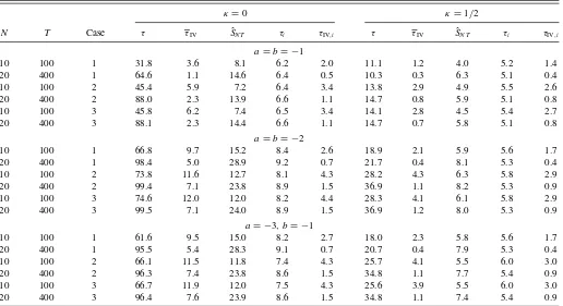
Table 2. Power at the 5% level
κ=0 κ=1/2
N T Case τ τIV SˆN T τi τIV,i τ τIV SˆN T τi τIV,i
a=b= −1
10 100 1 31.8 3.6 8.1 6.2 2.0 11.1 1.2 4.0 5.2 1.4 20 400 1 64.6 1.1 14.6 6.4 0.5 10.3 0.3 6.3 5.1 0.4 10 100 2 45.4 5.9 7.2 6.4 3.4 13.8 2.9 4.9 5.5 2.6 20 400 2 88.0 2.3 13.9 6.6 1.1 14.7 0.8 5.9 5.1 0.8 10 100 3 45.8 6.2 7.4 6.5 3.4 14.1 2.8 4.5 5.4 2.7 20 400 3 88.1 2.3 14.4 6.6 1.1 14.7 0.7 5.8 5.1 0.8
a=b= −2
10 100 1 66.8 9.7 15.2 8.4 2.6 18.9 2.1 5.9 5.6 1.7 20 400 1 98.4 5.0 28.9 9.2 0.7 21.7 0.4 8.1 5.3 0.4 10 100 2 73.8 11.6 12.7 8.1 4.3 28.2 4.3 6.3 5.8 2.9 20 400 2 99.4 7.1 23.8 8.9 1.5 36.9 1.1 8.2 5.3 0.9 10 100 3 74.6 12.0 12.0 8.2 4.4 28.3 4.1 6.1 5.8 2.9 20 400 3 99.5 7.1 24.0 8.9 1.5 36.9 1.2 8.0 5.3 0.9
a= −3, b= −1
10 100 1 61.6 9.5 15.0 8.2 2.7 18.0 2.3 5.8 5.6 1.7 20 400 1 95.5 5.4 28.3 9.1 0.7 20.7 0.4 7.9 5.3 0.4 10 100 2 66.1 11.5 11.8 7.4 4.3 25.7 4.1 5.5 6.0 3.0 20 400 2 96.3 7.4 23.8 8.6 1.5 34.8 1.1 7.7 5.4 0.9 10 100 3 66.7 11.9 12.0 7.5 4.3 25.6 3.9 5.5 6.0 3.0 20 400 3 96.4 7.6 23.9 8.6 1.5 34.8 1.1 7.4 5.4 0.9
NOTES:κ,aandbare such thatρi=exp(ci/NκT), whereci∼U(a, b). SeeTable 1for anexplanation of the rest.
statistics are constructed ast-ratios of the null hypothesis of
a unit root. The difference is that while the first is a time series test, the second is a panel test. Thus, the most relevant
compar-ison here is betweenτiandτIV,i, on the one hand, and between
τ andτIV, on the other hand. Moreover, in view of the
appar-ent robustness of the sign function to heteroscedasticity (see
Demetrescu and Hanck 2011, Proposition 1), the sign-based ˆ
SN T statistic, which in construction is very close toτIV, is also
simulated. A number of other tests were attempted (including
the ADFceˆ(i) andPeˆcstatistics ofBai and Ng 2004)but not
in-cluded, as their performance was dominated by the performance
of the above tests.9
In the simulations, the groups and lag augmentation order
are selected as described in Section3.3, using the QML and
MBIC, respectively. Consistent with the results ofNg and Perron
(1995), the maximum number of lags is set equal to pmax=
⌊4(T /100)2/9⌋. All tests are based on the same lag augmentation.
The trimming parameter in the QML is set toq =0.15 (see, e.g.,
Bai 1997). The number of factors are determined using theI C1
information criterion ofBai and Ng (2002)with the maximum
Shin and Kang (2006), in which the data are weighted by the inverse of the conventional estimator of the cross-sectional covariance matrix of the errors. The second test is based on a modified covariance matrix estimator that is supposed to work better in small samples. The results were, however, very similar, and we therefore only report the results from the latter test. Also, the test that we denote here byτIV,i is the weighted time series test that is used
in constructingτIV. WhileDemetrescu and Hanck (2011)did not present any asymptotic results for this test, in view of their Proposition 2, it seems reasonable to expect it to share the robustness ofτIV.
9SeeDemetrescu and Hanck (2011, sec.4) for a comprehensive Monte Carlo
comparison with their tests.
number of factors set to ⌊4(min{N, T}/100)2/9
⌋(Bai and Ng 2004).
The results are reported in Tables1–3.Table 1contains the
size results, while Tables 2 and3 contain the power results.
The information content of these tables may be summarized as follows.
• As expected, τi and τ are generally correctly sized. Of
course, the accuracy is not perfect, and some distortions remain. In particular, both tests seem to have a tendency to reject too often. Fortunately, the distortions are never very
large, and they vanish quickly asNandT increase, which
is just as expected, becauseT > N (corresponding to the
requirement that asymptoticallyN/T should go to zero)
in the simulations. We also see that none of the tests seem
to be affected much by the specification ofσ2
t.
• The most serious distortions are found for τIV, which is
generally quite severely undersized, especially whenφ1=
0.5 and the errors are serially correlated. Of course, with
T =N2 the requirement thatT > N5 (corresponding to
N/T1/5
→0 asN, T → ∞) is not even close to being
satisfied, and therefore the poor performance ofτIVin this
case does not come as a surprise. There is also no tendency
for the distortions to become smaller asNandTincreases.
In fact, the distortions actually increase with the sample
size. τIV,i is also undersized, although not to the same
extent asτIV.
• Whenκ =0 the power ofτ is increasing in the sample
size, which is to be expected, as the rate of shrinking of the local alternative in this case is not fast enough to prevent
the test statistic from diverging withN. The same reasoning
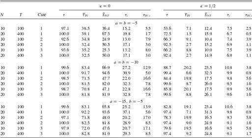
Table 3. Power at the 5% level
κ=0 κ=1/2
N T Case τ τIV SˆN T τi τIV,i τ τIV SˆN T τi τIV,i
a=b= −5
10 100 1 97.1 38.5 36.4 15.2 5.5 53.6 7.1 12.4 7.5 2.5 20 400 1 100.0 39.1 67.3 19.8 1.7 72.5 1.5 15.9 6.7 0.5 10 100 2 92.6 34.8 24.9 13.0 7.9 66.3 9.1 10.4 7.4 3.9 20 400 2 100.0 32.4 50.5 17.1 3.0 92.5 2.7 15.2 6.9 1.1 10 100 3 93.6 35.2 25.3 13.2 8.0 66.2 8.8 10.0 7.5 3.9 20 400 3 100.0 32.5 50.0 17.1 3.0 92.4 2.7 14.9 6.9 1.1
a=b= −10
10 100 1 99.6 83.4 66.9 27.2 12.9 88.7 20.2 23.5 10.8 3.8 20 400 1 100.0 91.7 94.6 39.9 5.0 99.4 6.6 32.3 9.9 0.8 10 100 2 98.5 71.5 47.7 22.0 16.6 84.4 19.8 17.5 9.8 5.6 20 400 2 100.0 81.5 82.0 32.3 7.8 99.6 8.7 26.0 9.5 1.6 10 100 3 98.7 70.8 47.1 22.8 16.6 85.8 20.1 17.5 9.9 5.6 20 400 3 100.0 81.8 81.9 32.8 7.8 99.6 8.8 26.1 9.6 1.6
a= −15, b= −5
10 100 1 99.6 83.1 65.8 25.2 13.9 82.8 19.1 23.4 10.6 3.8 20 400 1 100.0 92.2 93.6 37.1 5.6 97.4 7.1 31.3 9.8 0.8 10 100 2 97.1 71.8 48.0 20.2 17.0 78.3 19.9 16.5 9.3 5.8 20 400 2 100.0 82.5 81.8 28.9 8.5 97.4 9.0 24.9 9.1 1.6 10 100 3 97.9 72.0 47.6 20.7 17.1 79.6 19.5 16.6 9.5 5.8 20 400 3 100.0 82.8 81.9 29.3 8.5 97.4 9.2 24.8 9.1 1.7
NOTES: See Tables1and2for an explanation.
should in principle apply toτIV. However, this is not what
we observe. In fact, on the contrary, unless a andb are
relatively large in absolute value, the power of this test is actually decreasing in the sample size, which again is
probably becauseT < N5. The choiceκ
=1/2 is similarly
too fast forτiandτIV,ito have nonnegligible power.
• Whenκ =0 the power of the time series tests increases
slightly in T, and for the panel tests there is a
corre-sponding power increase in NandT whenκ =1/2. For
larger sample sizes, however, the power is quite flat in
N andT, which is in accordance with our expectations,
since for these combinations of tests and values ofκthere
should be no dependence on the sample size, atleast not asymptotically.
• The best power among the time series tests is obtained by
usingτi, and among the panel testsτis clearly the preferred
choice. Of course, given their size distortions under the null and the fact that the reported powers are not size-adjusted,
τIV,iandτIVare actually expected not to perform as well
as the new tests. However, the difference in power is way larger than the required compensation for size. In fact, it is not uncommon for the power of the new tests to be more than two times as powerful as the other tests. To take
an extreme example, consider the case whenκ =1/2 and
a=b= −5, in which the power ofτcan be up to 30 times
larger than that ofτIV!
• Power depends on the nature of the heteroscedasticity. This
is particularly clear whenκ =1/2,a= −3 andb= −1,
in which case the power ofτraises from about 20% in case
1 to about 30% in cases 2 and 3, which is just as expected
based on the example given in Section 3.2. Unreported
results suggest that there is also some variation in power coming from the location of the variance break, which is again in accordance with our expectations.
• The power ofτ when a=b= −2 anda =b= −10 is
about the same as whena= −3 andb= −1, anda= −15
andb= −5, respectively, which confirms the theoretical
prediction that the power of this test should be driven
mainly byμc. However, there is also a slight tendency for
power to decrease as we go froma =b= −10 toa= −15
andb= −5, although the effect vanishes asN andT
in-crease. This is in agreement with Theorem 2, suggesting that there should be a second-order effect working through
σ2
c.
The results reported in Tables1–3are just a small fraction
of the complete set of results that was generated. Some of the results that for space constraints are not reported here, most of which pertains to the selection of the groups, can be found in the supplement. The following summarizes the findings based on those results:
• The QML group selection approach works very well in
small samples.
• The “cost” in terms of test performance of having to
esti-mate the groups is very small. Indeed, the size and power results based on known groups are almost identical to the
ones reported in Tables1–3.
• As pointed out by a referee, whenNm−Nm−1=1, such
that the number of groups is equal toN, then Rˆwi,t =
ˆ
wi,tǫˆi,t =sign( ˆǫi,t), and sign-based tests have been shown
to be robust to certain types of heteroscedasticity (see
Demetrescu and Hanck 2011). Hence, while our theoretical results require that the size of each group goes to infinity
withN, the new tests are still expected to perform quite
well even when the groups are very small, and this is also what we find.
• While size accuracy is basically unaffected by the size of
the groups, as expected, accounting for the group structure can lead to substantial gains in power.
All-in-all, the results reported here and in the supplement lead to us to conclude that the new tests perform well in small samples, and also when compared to some of the existing tests. They should therefore be a valuable addition to the already existing menu of panel unit root tests.
5. CONCLUDING REMARKS
This article focuses on the problem of how to test for unit roots in panels where the errors are contaminated by time series and cross-section dependence, and in addition general uncon-ditional heteroscedasticity. In the article, we assume that the heteroscedasticity is deterministic, as when considering mod-els of permanent shifts or linear time trends, but it could also be stochastic. Conditional heteroscedasticity in the form of, for example, GARCH is permitted too. Moreover, the heteroscedas-ticity is not restricted to time series dimension, but can also em-anate to some extent from the cross-sectional dimension. The assumed DGP is therefore very general, and much more so than in most other panel data studies. In fact, the only other panel study that we are aware of to consider such a general setup is
that ofDemetrescu and Hanck (2011).
Two tests are proposed. One is designed to test for a unit root in a single cross-section unit, while the other is designed to test for a unit root in the whole panel. Both tests are re-markably simple, requiring no prior knowledge regarding the heteroscedasticity, and still only minor corrections are needed to obtain asymptotically nuisance parameter free test distribu-tions. This invariance is verified in small samples using Monte Carlo simulation. It is found that the new tests show smaller size
distortions than the tests ofDemetrescu and Hanck (2011)and,
at the same time, have much higher power. These findings sug-gest that they should be a useful addition to the existing menu of unit root tests.
APPENDIX: PROOFS
Lemma A.1. Under Assumptions 1–3,
Rˆwi,t =Rwi,t+gi,t+Op
1
C2N T
,
1
√
T
ˆ
Rwi,t =
1
√
T(Rwi,t+Gi,t)+Op
1
C2N T
,
where
Rwi,t =εi,t+(ρi−1)wm,tRi,t−1,
Rwi,t = t
s=pi+2
εi,s+(ρi−1) t
s=pi+2
wm,sRi,s−1,
gi,t =′iH−
1w
m,tvt−
1
2w
3
m,t(c0m,t+c4m,t+c6m,t)εi,t,
Gi,t =′iH−
1
t
s=pi+2
wm,svs−
1 2
t
s=pi+2
w3m,sc0m,sεi,s,
csm,t =
1
(Nm−Nm−1)
Nm
i=Nm−1+1 csi,t,
with i=Nm−1+1, . . . , Nm, Ri,t=φi(L)ui,t, c0i,t=(ǫ2i,t−
σm,t2 ), c4i,t =2ǫi,tai,t, c6i,t= −2( ˆi−i)′ǫi,txi,t−1, ai,t=
′
iH−1vt−di′Fˆt, vt =( ˆFt−H Ft), di =( ˆi−(H−1)′i),H
is ar×rpositive definite matrix andC2N T =min{N,
√
T}. Proof of Lemma A.1. Letxi,t=(yi,t, . . . , yi,t−p+1)′andi =
(φ1i, . . . , φpi)′. We have
Ri,t=φi(L)ui,t=φi(L)(yi,t−αi)=yi,t−′ixi,t−1−φi(1)αi,
whose first difference is given by
Ri,t=φi(L)yit=yi,t−′ixi,t−1.
It follows that
Ri,t =(ρi−1)Ri,t−1+ei,t, (A.1)
whereei,tis defined in Equation (4).
ConsiderRˆi,t, which we can expand as
Rˆi,t=yi,t−ˆ′ixi,t−1=Ri,t−( ˆi−i)′xi,t−1.
Note that by Taylor expansion of exp(x) about x =0,
exp(x)=1+x+o(1), suggesting that ρi=exp(ci/NκT)=
1+ci/NκT +op(1). This implies
1
√
T
T
t=pi+2
xi,t−1Ri,t=
ci
NκT3/2
×
T
t=pi+2
xi,t−1Ri,t−1+
1
√
T
T
t=pi+2
xi,t−1ei,t+op(1).
In the proof of Theorem 1, we show thatRi,t−1/
√
T satisfies an
invariance principle, and therefore that the first term on the
right-hand side isOp(1/Nκ
√
T). As for the second term, by the Wold
decomposition, 1/φ(L) can be expanded asφ∗(L)=1/φ(L)=
∞
j=0φj∗Ljwithφ0∗=1. It follows that,yi,t =(ρi−1)(yi,t−
αi)+vi,t, where vi,t =φi∗(L)ei,t. Hence, sinceei,t is serially
uncorrelated, we have thatE(ei,sxk,s−1)=0 for all i,kand
s. The variance ofT
t=pi+2xi,t−1ei,t/
√
T is bounded. Hence,
T
t=pi+2xi,t−1ei,t/
√
T =Op(1). Subsequently, using ˆi to
denote the OLS estimator ofi,
√
T( ˆi−i)=
⎛
⎝
1
T
T
t=pi+2
xi,t−1(xi,t−1)′
⎞
⎠
−1
×√1
T
T
t=pi+2
xi,t−1Ri,t
=
⎛
⎝
1
T
T
t=pi+2
xi,t−1(xi,t−1)′
⎞
⎠
−1
×√1
T
T
t=pi+2
xi,t−1ei,t+op(1)=Op(1).
The presence of the factors therefore does not affect the rate of
consistency of ˆi. Making use of this result, we obtain
Rˆi,t=yi,t−ˆ′ixi,t−1=Ri,t−( ˆi−i)′xi,t−1
=Ri,t+Op
1
√
T
, (A.2)
and therefore, with Ri,t−1=Op(
√
T) and (ρi−1)=
Op(1/NκT),
Rˆi,t =Ri,t+Op
1
√
T
=ei,t+(ρi−1)Ri,t−1
+Op
1
√
T
=ei,t+Op
1
√
T
. (A.3)
Sinceei,t =′iFt+ǫi,t, we have that the error incurred by
ap-plying the principal components method toRˆi,trather than to
ei,tis negligible (a detailed proof is available upon request). To
also show that the estimation is unaffected by the
heteroscedas-ticity inǫi,t, we verify Assumption C inBai (2003). Toward this
end, note that, sinceNm= ⌊λmN⌋,
1
N
N
i=1
E ǫ2i,t
=
M+1
m=1
(Nm−Nm−1)
N
1
(Nm−Nm−1)
Nm
i=Nm−1+1 E ǫ2i,t
=
M+1
m=1
(λm−λm−1)
1
(Nm−Nm−1)
Nm
i=Nm−1+1 E ǫi,t2
=
M+1
m=1
(λm−λm−1)σm,t2 ,
which is bounded under our assumptions, and therefore so is
N
i=1
N
j=1E(ǫi,tǫj,t)/N =Ni=1E(ǫi,t2)/N. Similarly,
1
N T
N
i=1
N
j=1
T
t=1
T
s=1
E(ǫi,tǫj,s)
= N T1
T
t=1
N
i=1
E ǫi,t2= 1 T
T
t=1
M+1
m=1
(λm−λm−1)σm,t2 ,
which is bounded too, becauseT
t=1σ 2
m,t/T →
1
r=0σ 2
m(r)dr
<∞ as T → ∞. Similarly, since 1
r=0 (r)dr >0,
T
t=1
FtFt′/T converges to a positive definite matrix. These results
imply that Assumption C ofBai (2003)holds and therefore that
the principal component estimators ˆi and ˆFt of ′i and Ft,
respectively, are unaffected by the heteroscedasticity.
Let us now considerRˆwi,t =wˆm,tǫˆi,t =ǫˆi,t/σˆm,t. Here,
ˆ
ǫi,t =eˆi,t−ˆ′iFˆt=ǫi,t+(ρi−1)Ri,t−1+ai,t
−( ˆi−i)′xi,t−1, (A.4)
where, followingBai and Ng (2004, p. 1154),
ai,t =′iFt−ˆ′iFˆt =′iH−
1
( ˆFt−H Ft)−( ˆi−(H−1)′i)′
ˆ
Ft =′iH−
1v
t−di′Fˆt,
withvt anddi implicitly defined. Hence,
ˆ
ǫi,t2 =(ǫi,t+(ρi−1)Ri,t−1+ai,t−( ˆi−i)′xi,t−1)2
=ǫi,t2 +c1i,t+ · · · +c9i,t, (A.5)
where
c1i,t =(ρi−1)2Ri,t2−1,
c2i,t =a2i,t,
c3i,t =( ˆi−i)′xi,t−1xi,t′ −1( ˆi−i),
c4i,t =2ǫi,tai,t,
c5i,t =2(ρi−1)ǫi,tRi,t−1,
c6i,t = −2( ˆi−i)′ǫi,txi,t−1,
c7i,t =2(ρi−1)ai,tRi,t−1,
c8i,t = −2( ˆi−i)′ai,txi,t−1,
c9i,t = −2(ρi−1)( ˆi−i)′Ri,t−1xi,t−1.
For ease of notation and without loss of generality, in what
follows we focus on the first group containing the first N1
cross-section units. Let us therefore consider ˆσ2
1,t, which is
ˆ
σ2
m,t for the first group. Letting c0i,t=(ǫi,t2 −σ12,t) and using
cs1,t = N1
i=1csi,t/N1to denote the averagecsi,t for this group,
we have
ˆ
σ12,t = 1 N1
N1
i=1
ˆ
ǫi,t2 = 1 N1
N1
i=1
ǫi,t2 +c11,t+ · · · +c91,t
=σ12,t+c01,t+ · · · +c91,t =σ12,t +C1,t, (A.6)
with an obvious definition ofC1,t. This result, together with a
second-order Taylor expansion of the inverse square root of ˆσ12,t,
yields
ˆ
w1,t =
1 ˆ
σ1,t
=w1,t −
1
2w
3 1,t σˆ
2 1,t−σ
2 1,t
+3
4w
5 1,t σˆ
2 1,t−σ
2 1,t
2
+Op
ˆ
σ12,t −σ12,t3
=w1,t −
1
2w
3 1,tC1,t +
3
4w
5 1,tC
2
1,t+Op C
3 1,t
. (A.7)
To work out the order of the remainder, we are going to make
use of Lemma 1 of Bai and Ng (2004), which states that
||vt|| =Op(1/C1N T) and||di|| =Op(1/C2N T), whereC1N T =
min{√N , T}andC2N T =min{N,
√
T}.
Remark A.1. The expansion in Equation (A.7) has to be of second order, because otherwise the resulting remainder
in the numerator of τ, N would not necessarily be negligible. For the numerator of
τi, Tt=pi+2Rˆwi,tRˆwi,t−1/T, it is enough with a first-order
1,t)=0, cross-section
indepen-dence andN1=λ1N =O(N). As forc21,t, by using (a+b)2≤
ǫi,tdivt, where, by the Cauchy–Schwarz inequality,
It follows that
and so, via the cross-section independence ofǫi,t,
|c41,t| =
of these are as follows:
c51,t =
substitution of Equations (A.8)–(A.12) into the definition of
C1,t,
where the order of the remainder follows from the fact that
Op
The result in Equation (A.16) suggests that Rˆi,t can be
ex-panded as
Rˆwi,t =wˆ1,tǫˆi,t
=wˆ1,t(ǫi,t+(ρi−1)Ri,t−1+ai,t−( ˆi−i)′xi,t−1)
=Rwi,t+w1,t(ai,t−( ˆi−i)′xi,t−1)
−1
2w
3
1,tC1,tRwi,t
−1
2w
4
1,tC1,t(ai,t−( ˆi−i)′xi,t−1)
+3
4w
5 1,tC
2 1,tRwi,t
+3
4w
6 1,tC
2
1,t(ai,t−( ˆi−i)′xi,t−1)+Op
1
CN T3
,
(A.17)
whereRwi,t =εi,t+(ρi−1)w1,tRi,t−1. Consider the second
term on the right-hand side,w1,t(ai,t−( ˆi−i)′xi,t−1). By
using ai,t=′iH−
1v
t−di′Fˆt =′iH−
1v
t+Op(1/C2N T) and
|( ˆi−i)′xi,t−1| ≤ ||ˆi−i||||xi,t−1|| =Op(1/
√
T )=
Op(1/C2N T), it is clear that
w1,t(ai,t−( ˆi−i)′xi,t−1)=′iH−
1w
1,tvt+Op
1
C2N T
.
The order ofC1,tRwi,tis equal to that ofC1,t, and therefore
C1,tRwi,t =(c01,t+c41,t+c61,t)Rwi,t+Op
1
C2
N T
.
Similarly, sinceC1,t andai,tare bothOp(1/CN T),
|C1,t(ai,t−( ˆi−i)′xi,t−1)|
≤ |C1,t|(|ai,t| − ||ˆi−i||||xi,t−1||)
=Op
1
CN T2
+Op
1
√
T CN T
,
which is clearlyOp(1/C2N T). The other terms are all of higher
order than this. It follows that
Rˆwi,t =Rwi,t+′iH−
1
w1,tvt−
1
2w
3
1,t(c01,t +c41,t+c61,t)
×Rwi,t+Op
1
C2N T
=Rwi,t+′iH−
1
w1,tvt−
1
2w
3
1,t(c01,t+c41,t+c61,t)εi,t
+Op
1
C2N T
=Rwi,t+gi,t+Op
1
C2N T
, (A.18)
with an obvious definition ofgi,t, and where the second equality
uses the approximation Rwi,t =εi,t+(ρi−1)w1,tRi,t−1=
εi,t+op(1), which is valid in the present case (details are
avail-able upon request). This establishes the first of the two required results.
The second result requires more work. Note first that by using
Equation (A.16),
1
√
T
ˆ
Rwi,t
=√1
T
t
s=pi+2
Rˆwi,s
=√1
TRwi,t+
1
√
T
t
s=pi+2
w1,s(ai,s−( ˆi−i)′xi,s−1)
− 1
2√T
t
s=pi+2
w31,sC1,sRwi,s
− 1
2√T
t
s=pi+2
w41,sC1,s(ai,s−( ˆi−i)′xi,s−1)
+ 3
4√T
t
s=pi+2
w51,sC21,sRwi,s
+ 3
4√T
t
s=pi+2
w61,sC21,s(ai,s−( ˆi−i)′xi,s−1)
+Op
√T C3
N T
, (A.19)
where again all terms that areOp(1/C2N T) can be treated as
negligible.
Consider t
s=pi+2w1,s(ai,s−( ˆi−i)
′xi,s −1)/
√
T.
Via ˆFs =HFs+vs, and then leading term approximation,
t
s=pi+2w1,sFˆs/
√
T =t
s=pi+2w1,sHFs/
√
T +op(1)=Op
(1), implying
1
√
T
t
s=pi+2
w1,sais
=′iH−1√1 T
t
s=pi+2
w1,svs−di′
1
√
T
t
s=pi+2
w1,sFˆs
=′iH−1√1 T
t
s=pi+2
w1,svs+Op
1
C2N T
,
which, together with ( ˆi−i)′ts=pi+2w1,sxi,s−1/
√
T = Op(1/
√
T ), yields
1
√
T
t
s=pi+2
w1,s(ai,s−( ˆi−i)′xi,s−1)=′iH−
1 1
√
T
×
t
s=pi+2
w1,svs+Op
1
C2N T
. (A.20)
Next, consider
T is again not of
suffi-ciently low order to be ignored. Let us therefore consider
t
s=pi+2w
3
1,sc61,sRwi,s/
√
T. Becauseǫi,tis serially
uncorre-lated and independent ofFt, we haveE(εi,sxk,s−1)=0.
More-Similarly, sincet
s=pi+2w
3
1,sεk,sxk,s−1Ri,s−1/T3/2=Op(1),
we can show
(ρi−1)
T. We now verify that the remaining
terms in Equation (A.21) are negligible too. In so doing, note
that, as in the above, the effect of (ρi−1)w1,sRi,s−1 inRwi,s
will generally be dominated by that ofεi,s. Hence, unless
oth-erwise stated, in what follows we are going to work with the
approximationRwi,s=εi,s+op(1).
BothRi,t/
√
T andRwi,t/
√
T satisfy an invariance principle.
By using this and the fact that (ρi−1)=Op(1/NκT),
It is also not difficult to show that
and similarly,
The terms involvingai,tcan be evaluated in a similar fashion.
In particular, we have
p. 1158), from which we deduce that t
s=pi+2ak,s/
op(1), whereεi,tis asymptotically uncorrelated with ˆFt,
1
As for the remaining term, according to Bai (2003,
p. 166), vs =H′−1
is cross-section independent, we obtain
1
=H′−1√1
from which it follows that
1
third equality holds because
The remaining term can be written as
1