07350015%2E2012%2E634340

Full Terms & Conditions of access and use can be found at

http://www.tandfonline.com/action/journalInformation?journalCode=ubes20

Download by: [Universitas Maritim Raja Ali Haji] Date: 11 January 2016, At: 22:25

Journal of Business & Economic Statistics

ISSN: 0735-0015 (Print) 1537-2707 (Online) Journal homepage: http://www.tandfonline.com/loi/ubes20

Comment

Dean Croushore

To cite this article: Dean Croushore (2012) Comment, Journal of Business & Economic Statistics, 30:1, 17-20, DOI: 10.1080/07350015.2012.634340

To link to this article: http://dx.doi.org/10.1080/07350015.2012.634340

Published online: 22 Feb 2012.

Submit your article to this journal

Article views: 171

[14]

Nordhaus, W. D. (1987), “Forecasting Efficiency: Concepts and Applications,” Review of Economics and Statistics, 69, 667–674. [2]

Patton, A. J., and Timmermann, A. (2007a), “Properties of Optimal Forecasts under Asymmetric Loss and Nonlinearity,”Journal of Econometrics, 140, 884–918. [1]

——(2007b), “Testing Forecast Optimality under Unknown Loss,”Journal of the American Statistical Association, 102, 1172–1184. [14]

—— (2010a), “Monotonicity in Asset Returns; New Tests with Applications to the Term Structure, the CAPM, and Portfolio Sorts,”Journal of Financial Economics, 98 , 605–625. [3]

——(2010b), “Why do Forecasters Disagree? Lessons from the Term Structure of Cross-sectional Dispersion,”Journal of Monetary Economics, 57, 803– 820. [2]

——(2011), “Predictability of Output Growth and Inflation: A Multi-horizon Survey Approach,”Journal of Business and Economic Statistics, 29, 397– 410. [2]

Pesaran, M. H. (1989), “Consistency of Short-Term and Long-Term Ex-pectations,” Journal of International Money and Finance, 8, 511– 516. [4]

309. [2]

Sun, H.-J. (1988), “A General Reduction Method for n-Variate Nor-mal Orthant Probability,” Communications in Statistics, 17(11), 3913– 3921. [3]

West, K. D. (1996), “Asymptotic Inference about Predictive Ability,” Econo-metrica, 64, 1067–1084. [2]

West, K. D., and McCracken, M. W., “Regression Based Tests of Predictive Ability,”International Economic Review, 1998, 39, 817–840. [2] White, H. (2000), “A Reality Check for Data Snooping,”Econometrica, 68,

1097–1126. [1]

White, H. (2001), Asymptotic Theory for Econometricians(2nd ed), San Diego: Academic Press. [8]

Wolak, F. A. (1987), “An Exact Test for Multiple Inequality and Equality Con-straints in the Linear Regression Model,”Journal of the American Statistical Association, 82, 782–793. [1]

——(1989), “Testing Inequality Constraints in Linear Econometric Models,” Journal of Econometrics, 31, 205–235. [1]

Wooldridge, J. M., and White, H. (1988), “Some Invariance Principles and Central Limit Theorems for Dependent Heterogeneous Processes,” Econo-metric Theory, 4, 210–230. [8]

Comment

Dean C

ROUSHORE

Economics Department, University of Richmond, Richmond, VA 23173-0002, and Federal Reserve Bank of Philadelphia, Philadelphia, PA 19106-1574 (dcrousho@richmond.edu)

In the forecasting literature, researchers often seek to deter-mine stylized facts, such as: Are forecasts rational? But fore-casts can be characterized in many dimensions and answering the question about whether forecasts are rational may require a multidimensional answer. I think about forecasts in three di-mensions: (1) horizon, (2) subsample, and (3) vintage.

One dimension of forecast rationality is the horizon of the forecast. The literature on the rationality of forecasts finds some differences across forecast horizons. Zarnowitz (1985) found that the results of tests for bias vary across horizons with no systematic tendency across variables, using individual fore-casts from the ASA-NBER (American Statistical Association– National Bureau of Economic Research) survey (now the Survey of Professional Forecasters, SPF). Similarly, Brown and Maital (1981) found varying bias across horizons for forecasts of vari-ables from the Livingston survey. Generally, the early literature in the 1980s finds many cases of bias in forecasts. However, Keane and Runkle (1990) found convincing evidence of no bias for inflation at short horizons using the individual forecasters in the ASA-NBER survey.

The second dimension of forecast rationality is the subsam-ple. Though researchers seek to find stylized facts, they are thwarted by instabilities in empirical results across subsamples. Croushore (2010) shows how forecast rationality tests using SPF forecasts change dramatically over time, depending on the starting date and ending date of the subsample. For example,

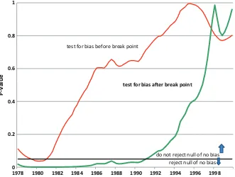
Figure 1shows how the sample ending date affects the results of a rationality test, which is a test that determines whether the mean forecast error is zero. The plot shows thep-value testing

the null hypothesis whether the mean forecast error is zero for different subsamples. The line labeledtest for bias before break pointshows thep-values for tests using subsamples that begin in 1971 and end at the date shown on the horizontal axis. The line labeledtest for bias after break pointshowsp-values for tests using subsamples that begin at the date shown on the hori-zontal axis and end at the end of 2008. The idea is that when we look for stylized facts, we are limited by the data available to us. And the starting and ending dates of our samples are often random or occur by happenstance. Suppose the development of the SPF had been delayed 5 or 10 years; then we would have a very different starting date for many of our forecast tests. If the facts we discover are truly stylized facts, then they should not be affected by small changes in the starting or ending dates of our data series. However, a look atFigure 1suggests that facts about the rationality of SPF inflation forecasts are a function of the subsample. Depending on the exact starting or ending dates of the sample, we reach different conclusions about the rationality of the survey forecasts. Thus, no stylized fact is found that is robust across subsamples.

The third dimension of forecast rationality is the data vin-tage. Croushore (2011) shows that the results of some fore-cast rationality tests depend somewhat on the vintage of the data chosen as “actual” to be used to evaluate the accuracy of

© 2012American Statistical Association Journal of Business & Economic Statistics

January 2012, Vol. 30, No. 1 DOI:10.1080/07350015.2012.634340

0 0.2 0.4 0.6 0.8 1

1978 1980 1982 1984 1986 1988 1990 1992 1994 1996 1998

P-value

reject null of no bias do not reject null of no bias test for bias before break point

test for bias aer break point

Figure 1. p-values for bias at alternative break dates. The plot shows thep-value testing the null hypothesis that the mean forecast error is zero for different subsamples. The line labeledtest for bias before break pointshows thep-values for tests using subsamples that begin in 1971 and end at the date shown on the horizontal axis. The line labeledtest for bias after break pointshowsp-values for tests using subsamples that begin at the date shown on the horizontal axis and end at the end of 2008. (Color figure available online.)

forecasts. Many data series are revised for very long periods of time, so how does a researcher choose which measure to use? In the literature, the choices have varied from the release of data two months after the initial release, to the annual revision, to the last vintage before a benchmark revision, to the latest-available data series. But that seemingly innocuous choice may have a large impact on tests for rationality. For example,Figure 2

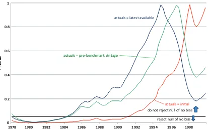
shows the sensitivity of the zero-mean forecast error test to the choice of both the starting date of the forecast (shown on the horizontal axis) and the choice of variable used as actual (ini-tial, pre-benchmark, or latest-available). Clearly, not only does the subsample period affect the rationality test, but so does the choice of actual. Choosing the initial actual leads to many more subsamples in which we reject the null hypothesis of no bias than using the other two choices of actuals.

In their article, “Forecast Rationality Tests Based on Multiple-Horizon Bounds,” Patton and Timmermann (2011) handle two of the three dimensions of forecast rationality tests: they look across alternative forecast horizons and they develop tests for which choosing an “actual” is not needed. They do not, however, look at the sensitivity of their results to alternative subsamples. The Patton–Timmermann article accomplishes two main ob-jectives. First, it uses forecasts across alternative horizons, which is valuable because theory implies restrictions on forecasts across different horizons that can be tested. The use of many dif-ferent horizons avoids issues about choosing which one horizon to analyze. Second, the article develops some tests for which no choice of actual is necessary, which is valuable in avoiding having to choose a vintage of the data to use as actual. Many researchers struggle with this issue. They often use as actuals the latest-available data, which is convenient, but which may be problematic because of re-definitions and other methodolog-ical changes. Alternatively, they must develop a real-time dataset

with some version of actual data that are not subject to distortions because of methodological changes if the data they need are not conveniently available in an existing real-time dataset, such as the Philadelphia Fed’s Real-Time Data Set for Macroeconomists (see Croushore and Stark2001). With the Patton–Timmerman tests, no choice of actual is necessary, so researchers avoid having to make this difficult choice. Forecasts, as well as data that will be revised in the future, are treated in a similar manner.

The article provides tests that are easy to interpret, because they lend themselves to graphical interpretations. For example,

Figure 1in the Patton–Timmermann article shows mean squared errors and variances of forecasts from the Greenbook. The sum of the two components should be constant across horizons if the forecasts are optimal, but the graph shows clearly that is not the case. In addition, the variance of the forecasts should increase with horizon if the forecasts are optimal, but that does not hold for the inflation series, as a quick glance at the figure illustrates.

Figure 2in the Patton–Timmermann article shows plots across horizons of mean squared forecast revisions and the covariance between the forecast and the actual (for this test, an actual must be chosen). Mean squared forecast revisions should increase as a function of horizon if the forecasts are optimal, but that is not the case for GDP growth. The covariance between the forecast and the actual should decrease with horizon if the forecasts are optimal, but that is not true for the GDP deflator.

So, the Patton–Timmermann article has many useful features and is the first to provide us with solid analytical results and easy-to-interpret tests. There are three issues about their methods that are worthy of further investigation: (1) The tests may not provide a researcher with the ability to engage in a forecast improvement exercise. (2) The assumptions of the article may not be valid when major benchmark revisions to the data occur. (3) The conclusions are potentially sensitive to the subsample choice.

0

reject null of no bias do not reject null of no bias

actuals = iniƟal

actuals = pre-benchmark vintage

Figure 2. Alternative actuals:p-values for bias after break point. The plot shows thep-value testing the null hypothesis that the mean forecast error is zero for different subsamples and different concepts of actuals. Each line showsp-values for tests using subsamples that begin at the date shown on the horizontal axis and end at the end of 2008. The line labeledactuals=initialshows thep-values for tests using as actuals the value recorded in the initial data release and is the same line as shown inFigure 1. The line labeledactuals=pre-benchmark vintageshows the

p-values for tests using as actuals the value recorded in the last vintage before a benchmark revision. The line labeledactuals=latest available

shows thep-values for tests using as actuals the value recorded in the vintage of May 2011. (Color figure available online.)

The first issue worthy of further investigation is that the tests may not provide a researcher with the ability to engage in a forecast improvement exercise. For example, consider the test discussed earlier for investigating whether mean forecast errors are zero. The mean forecast error iset =xta−x

f

t , where xta is the actual value andxtf is the forecast value. If we run the regressionet =α+εt, we can use the estimated value ofαto create an improved forecast:x_ti =α_ˆ+xtf, where the improved forecast isx_ti. Researchers in the 1980s who found bias in fore-casts advocated this procedure as a method to reduce forecast errors. Such a test can be used in many different contexts. For example, Faust, Rogers, and Wright (2005), used such a pro-cedure to show how that they can use initial data releases to forecast revisions to GDP in many countries, reducing the mean squared forecast error substantially.

The tests provided by Patton and Timmermann are useful in showing that forecasts are not optimal, but the tests do not lend themselves to forecast improvement possibilities. So, the tests can determine that there is a problem with the forecasts, but provide no guidance about what to do in response. Often in working on forecasts, we observe in-sample predictability of forecast errors, but we are unable to improve the forecasts in a real-time out-of-sample forecast improvement exercise. So, Patton and Timmermann might want to consider how to use their tests to provide guidance to forecasters on how to fix the problems their tests identify.

The second issue worth further investigation is that the as-sumptions in the article may not be valid under major bench-mark revisions to the data. In particular, the monotonicity of mean squared forecast revisions depends on the covariance

sta-tionarity of the data series. Under the benchmark revision pro-cess, forecast revisions that violate some of the proposed tests could be rational if large benchmark revisions cause a change in the data-generating process. Have such large revisions occurred in practice? It is hard to know for sure, but the Stark plots from Croushore and Stark (2001) are suggestive.

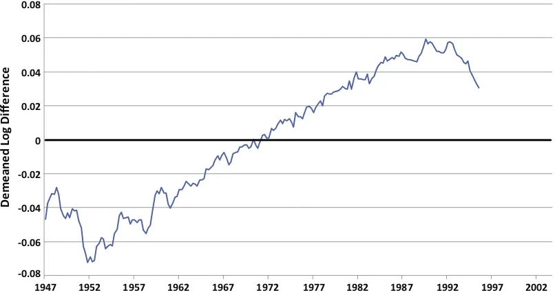
For example, Figure 3shows the Stark plot for the bench-mark revision of GDP in examining the key benchbench-mark revision that occurred in January 1996, which was the benchmark re-vision in which chain weighting was introduced and in which some government purchases were reclassified as investment. The plot shows the demeaned log differences of GDP before and after the benchmark revision of January 1996. It is a plot of log[X(t,b)/X(t,a)] –m, whereX(t,s) is the level ofX at date

t from vintage s, wheres=aor s=b,b >a, andmis the mean of log[X(τ,b)/X(τ,a)] for all the dates that are common to both vintagesaandb. The upward trend in the Stark plot means that later data were revised up more than earlier data. But the downward slope at the beginning and end of the sample shows a more complex pattern. This could cause a lack of covariance sta-tionarity across vintages and violate the conditions under which the monotonicity of mean squared forecast revisions is derived. Some work to ensure that this issue is not sufficient to worry about might be in order for data samples that include major benchmark revisions, such as that in 1996.

The third issue worth considering is that the conclusions could be sensitive to subsample choices. This may be worth investi-gating so that we do not falsely generalize about results based on the overall sample. Potentially, the tests proposed by Patton and Timmermann could be less sensitive to subsample choice

-0.08

Figure 3. Stark plot across January 1996 benchmark revision. The plot shows the demeaned log differences of GDP before and after the benchmark revision of January 1996. It is a plot of log[X(t,b)/X(t,a)] –m, whereX(t,s) is the level ofXat datetfrom vintages, wheres=aors =b,b>a, andmis the mean of log[X(τ,b)/X(τ,a)] for all the dates that are common to both vintagesaandb. In this plot,a=December 1995 andb=October 1999. (Color figure available online.)

than other tests, including the standard Mincer–Zarnowitz test and the test for zero-mean forecast errors.

To conclude, this article by Patton and Timmermann provides us with an excellent set of tests that can complement much existing research. The tests help us cross two dimensions of forecast rationality: horizon and real-time vintage. They could potentially help as well in the subsample dimension.

[Received April 2011. Revised August 2011.]

REFERENCES

Brown, B. W., and Maital, S. (1981), “What Do Economists Know? An Em-pirical Study of Experts’ Expectations,”Econometrica, 49, 491–504. [17]

Croushore, D. (2010), “An Evaluation of Inflation Forecasts From Surveys Using Real-Time Data,”B.E. Journal of Macroeconomics: Contributions, 10, 10. [17]

——— (2011), “Two Dimensions of Forecast Analysis,” Working Paper, Uni-versity of Richmond. [17]

Croushore, D., and Stark, T. (2001), “A Real-Time Data Set for Macroe-conomists,”Journal of Econometrics, 105, 111–130. [18,19]

Faust, J., Rogers, J. H., and Wright, J. H. (2005), “News and Noise in G-7 GDP Announcements,” Journal of Money, Credit, and Banking, 37, 403–419. [19]

Keane, M. P., and Runkle, D. E. (1990), “Testing the Rationality of Price Forecasts: New Evidence From Panel Data,”American Economic Review, 80, 714–735. [17]

Patton, A. J., and Timmermann, A. (2011), “Forecast Rationality Tests Based on Multi-Horizon Bounds,”Journal of Business and Economic Statistics, this issue. [18]

Zarnowitz, V. (1985), “Rational Expectations and Macroeconomic Forecasts,” Journal of Business & Economic Statistics, 3, 293–311. [17]

Comment

Kajal L

AHIRI

Department of Economics, University at Albany: SUNY, Albany, NY 12222 (klahiri@albany.edu)

1. INTRODUCTION

I enjoyed reading yet another article by Patton and Timmer-mann (PT hereafter) and feel that it has broken new ground in testing the rationality of a sequence of multi-horizon fixed-target forecasts. Rationality tests are not new in the forecasting literature, but the idea of testing the monotonicity properties of second moment bounds across several horizons is novel and can suggest possible sources of forecasting failure. The basic premise is that since fixed-target forecasts at shorter horizons

are based on more information, they should on the average be more accurate than their longer horizon counterparts. The inter-nal consistency properties of squared errors, squared forecasts, squared forecast revisions, and the covariance between the tar-get variable and the forecast revision are tested as inequality

© 2012American Statistical Association Journal of Business & Economic Statistics

January 2012, Vol. 30, No. 1 DOI:10.1080/07350015.2012.634342