Full Terms & Conditions of access and use can be found at
http://www.tandfonline.com/action/journalInformation?journalCode=ubes20
Download by: [Universitas Maritim Raja Ali Haji] Date: 13 January 2016, At: 01:06
Journal of Business & Economic Statistics
ISSN: 0735-0015 (Print) 1537-2707 (Online) Journal homepage: http://www.tandfonline.com/loi/ubes20
Bayes Estimates of Markov Trends in Possibly
Cointegrated Series
Richard Paap & Herman K Van Dijk
To cite this article: Richard Paap & Herman K Van Dijk (2003) Bayes Estimates of Markov Trends in Possibly Cointegrated Series, Journal of Business & Economic Statistics, 21:4, 547-563, DOI: 10.1198/073500103288619296
To link to this article: http://dx.doi.org/10.1198/073500103288619296
View supplementary material
Published online: 01 Jan 2012.
Submit your article to this journal
Article views: 65
Bayes Estimates of Markov Trends in Possibly
Cointegrated Series: An Application to
U.S. Consumption and Income
Richard P
AAPand Herman K.
VAND
IJKEconometric Institute, Erasmus University, Rotterdam
Stylized facts show that average growth rates of U.S. per capita consumption and income differ in reces-sion and expanreces-sion periods. Because a linear combination of such series does not have to be a constant mean process, standard cointegration analysis between the variables to examine the permanent income hypothesis may not be valid. To model the changing growth rates in both series, we introduce a multi-variate Markov trend model that accounts for different growth rates in consumption and income during expansions and recessions and across variables within both regimes. The deviations from the multivari-ate Markov trend are modeled by a vector autoregression (VAR) model. Bayes estimmultivari-ates of this model are obtained using Markov chain Monte Carlo methods. The empirical results suggest the existence of a cointegration relation between U.S. per capita disposable income and consumption, after correction for a multivariate Markov trend. This result is also obtained when per capita investment is added to the VAR.
KEY WORDS: Cointegration; Markov chain Monte Carlo; Multivariate Markov trend; Permanent in-come hypothesis.
1. INTRODUCTION
Thepermanent income hypothesisimplies that there exists a long-run relation between consumption and disposable income (see, e.g., Flavin 1981). This theoretical result may be trans-lated to time series properties. Most studies on the univariate properties of consumption and income series suggest that they are integrated processes (see the applications following Dickey and Fuller 1979). Hence both series must be cointegrated for the permanent income hypothesisto hold. As a result, recent empir-ical research on the permanent income hypothesis focuses on cointegration analysis between consumption and income (see, e.g., Campbell 1987; Jin 1995).
In these studies, it is usually assumed that the logarithm of real income is a linear process. However, Goodwin (1993), Pot-ter (1995), and Peel and Speight (1998), among others, have argued that the logarithm of many real income series contains a nonlinear cycle. This nonlinear cycle is often interpreted as the business cycle in real income. A popular model used to de-scribe the business cycle in time series is the Markov switching model of Hamilton (1989), which allows for different average growth rates in income during expansion and recession peri-ods, where the transitions between expansions and recessions are modeled by an unobserved rst-order Markov process. We refer to the trend that models this specic behavior as aMarkov trend. Hall, Psaradakis, and Sola (1997) considered the perma-nent income hypothesis under the assumption that real income contains a Markov trend. They showed that in this case, the dif-ference between log consumption and log income is affected by changes in the mean, caused by changes in the growth rate of the real income series. The difference between log consump-tion and income series is not a constant mean process such that standard cointegration analysis in linear vector autoregressive (VAR) models may wrongly indicate the absence of cointegra-tion (see Nelson, Piger, and Zivot 2001; Psaradakis 2001, 2002 for some results in univariate time series).
Several studies have considered the effects of deterministic shifts on cointegration relations (see, e.g., Gregory and Hansen
1996; Hansen and Johansen 1999; Martin 2000). In this arti-cle we analyze the long-run relationship between quarterly sea-sonally adjusted aggregate consumption and disposable income for the United States, where we allow for the possibility of a Markov trend in both the income and consumption series. Our work differs from previous studies in several ways. We consider a full system cointegration analysis in a nonlinear model. We test cointegration in a VAR, which models the deviation of log per capita consumption and income from a multivariate Markov trend. This differs from the approach of Hall et al. (1997), who considered a single equation analysis and used an ad hoc pro-cedure for cointegration analysis. Our model is a multivariate generalization of Hamilton’s (1989) model and nests the the-oretical results of Hall et al. (1997). Furthermore, the model allows the growth rate of consumption to be different from the growth rate in income at each stage of the business cycle, as suggested by a simple stylized facts analysis. Hence we ana-lyze the presence of a cointegration relation between consump-tion and income series while allowing for different growth rates in expansion and recession periods via the multivariate Markov trend. We investigate the robustness of our results by including an investment variable in the model.
To perform econometric inference on the presence of a stable long-run relation between per capita consumption and income, we follow a Bayesian approach. We apply Markov chain Monte Carlo (MCMC) methods to evaluate posterior distributions and construct Bayes factors (BFs) to determine the cointegration rank. Our Bayesian cointegration analysis is an extension of the techniques of Kleibergen and Paap (2002) and Kleibergen and van Dijk (1998) to the case of a nonlinear VAR model contain-ing a Markov trend.
The outline of the article is as follows. In Section 2 we give a short review on the current state of the literature on the per-manent income hypothesis in cases where income is assumed
© 2003 American Statistical Association Journal of Business & Economic Statistics October 2003, Vol. 21, No. 4 DOI 10.1198/073500103288619296 547
to contain a Markov trend. In Section 3 we discuss some styl-ized facts of U.S. per capita income and consumption series. In Section 4 we propose the multivariate Markov trend model and discuss its interpretation. Given the main application of this article, we limit the discussion to a bivariate model, but it can be easily extended to more dimensions, as shown in Section 9. In Section 5 we discuss prior specication, and in Section 6 we propose a MCMC algorithm to sample from the posterior distribution. We deal with BFs used to determine the cointegra-tion rank in Seccointegra-tion 7. In Seccointegra-tion 8 we apply our multivariate Markov model to the U.S. series and relate the posterior results to suggestions made by economic theory and the stylized facts analysis. To analyze the robustness of our results, in Section 9 we consider a Markov trend model for U.S. per capita income, consumption, and investment series. We conclude the article in Section 10.
2. THE PERMANENT INCOME HYPOTHESIS AND A MARKOV TREND
The permanent income hypothesis states that current aggre-gate consumption is equal to a weighted average of expected future real disposable incomes. More precisely, aggregate con-sumption,ct, can be written as
ctD
r 1Cr
1
X
jD0 1
.1Cr/jE[ytCjjÄt]; (1)
whereytis real disposable income at timet,ris the interest rate, andÄtdenotes the information set that is available to economic agents at timet. In Flavin’s (1981) formulation,ytdenotes labor income solely, in which case one must add real wealth to (1). We follow Sargent’s (1978) assumption that the annuity value of future capital income is equal to the value of real nan-cial wealth (see Flavin 1981 for a critique of this assumption). Straightforward algebra shows that (1) is the forward solution of the expectational difference equation
ctD
r
1CrE[ytjÄt]C 1
1CrE[ctC1jÄt]: (2)
Subtractingytfrom both sides of (1), we obtain
ct¡ytD
r
1Cr
1
X
jD0 1
.1Cr/jE[ytCj¡ytjÄt]; (3)
which shows that there exists a stationary relation between cur-rent consumption and income if the rst difference ofytis sta-tionary (see, e.g., Campbell 1987). In many studies it is there-fore assumed that real income follows a random-walk process (see, e.g., Jin 1995). Several other studies, however, suggest that the log income series contains a nonlinear cycle that cor-responds to the business cycle (see, e.g., Goodwin 1993; Potter 1995; Peel and Speight 1998). To capture this business cycle, one often assumes that log real income is the sum of a random-walk process and a Markov trend, as suggested by Hamilton (1989). To explain the role of the Markov trend on the perma-nent income hypothesis, we now briey discuss the approach of Hall et al. (1997).
The logarithm of real income is written as
lnytDntCzt; (4)
whereztis a standard random-walk process
ztDzt¡1C²t; (5)
with²t»NID.0; ¾2/ and where nt is a so-called univariate
Markov trend. This Markov trend is dened as
ntDnt¡1C°0C°1st; (6)
where°0and°1are parameters andstis an unobserved binary random variable that models the business cycle. In the remain-der of this article, we assume thatstD0 corresponds to an ex-pansion observation andstD1 corresponds to a recession. This implies that during an expansion, the slope of the Markov trend equals°0, whereas during a recession, the slope is given by
°0C°1. The random variablest is assumed to follow a rst-order, two-state Markov process with transition probabilities
Pr[stD0jst¡1D0]Dp; Pr[stD1jst¡1D0]D1¡p;
Pr[stD1jst¡1D1]Dq; Pr[stD0jst¡1D1]D1¡q (7)
(see Hamilton 1989 for details).
As Hall et al. (1997) showed, (2) and (4)–(6) with Ät D
fyt;yt¡1; : : : ;st;st¡1; : : :g imply thatctDe·0yt forstD0 and
ctDe·0C·1ytforstD1, with
·0Dln
³
rCpe·0E0C.1¡p/e·0C·1E1
1Cr
´
;
(8)
·0C·1Dln
³r
C.1¡q/e·0E
0Cqe·0C·1E1 1Cr
´
;
whereE0De°0C
1
2¾2 andE1De°0C°1C12¾2. Becausestis an
un-observed random process, we obtain the following relation be-tween log consumption and log income:
lnctD·0C·1stClnyt; (9)
where·0and·1result from (8); that is,
·0Dln
³ r.
1C.1¡p¡q/.1Cr/¡1E1/
.1Cr¡pE0¡qE1/¡.1Cr/¡1.1¡p¡q/E0E1
´
;
(10)
·1Dln
³
.1Cr/C.1¡p¡q/E0
.1Cr/C.1¡p¡q/E1
´
:
Substituting (4) in the consumption–income relation (9), we note that the log of consumption can be written as
lnctDntC·0C·1stCzt; (11)
whereztandntare dened in (5) and (6). It follows that log con-sumption is built up of the same Markov trend as log income, and hence it corresponds to the idea that growth rates of con-sumption and income are the same during expansions and reces-sions. Note that (4) and (11) with (5) and (6) imply a stochasti-cally singular system forytandct. To describe consumption and income series with this model, one must add extra noise to (11). Equation (9) implies that the difference between log consump-tion and log income is different across the phases of the busi-ness cycle and is described by the process wt D·0 C·1st. This process can be written aswtD¹C½wt¡1C·1vt, where
¹D.1¡½/·0C·1.1¡p/, ½D.¡1CpCq/, and vt is a martingale difference sequence (see Hamilton 1989). This im-plies that (9) can be seen as a cointegration relation between log consumption and income with non-Gaussian innovations. If the
transition probabilitiespandqare near 1 (i.e., if both regimes are persistent), then it may be difcult to distinguish the process wt from a random-walk process (see also Nelson et al. 2001; Psaradakis 2001, 2002). In turn, this may complicate detection of a stationary relation between log consumption and income using a standard cointegration analysis approach.
To test the presence of a stationary relation between U.S. log consumption and income, when the log of real income contains a Markov trend, we propose in Section 4 a multivariate Markov trend model. Because the economic theory in this section may be too simplistic in describing reality, we allow for a more ex-ible structure than the theory suggests. This exex-ible structure is based on a simple stylized facts analysis of the U.S. per capita income and consumption series given in the next section.
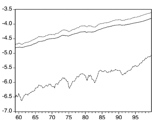
3. STYLIZED FACTS
Figure 1 shows a plot of the logarithm of quarterly observed seasonally adjusted per capita real disposable income and pri-vate consumption of the United States, 1959.1–1999.4. The se-ries were obtained from the Federal Reserve Bank of St. Louis. Both series are increasing over the sample period with short periods of decline, for example, in the middle and the end of the 1970s. These periods of decline are more pronounced in the income series than in the consumption series but seem to occur roughly simultaneously. The average quarterly growth rate of the income series is .67% per quarter. For the consump-tion series, the average quarterly growth rates equals .62%. The growth rates in both series seem roughly the same.
To analyze the effect of the business cycle on real per capita income and consumption, we split the sample in two subsam-ples. The rst subsample corresponds to quarters labeled a re-cession according to the National Bureau Economic of Re-search (NBER) peaks and troughs (see http://www.nber.org/ cycles.html). During recessions, the average quarterly growth rate of per capita income is¡1:03% and it is¡:24% for con-sumption. The second subsample contains quarters correspond-ing to expansion observations. Durcorrespond-ing expansions, the average quarterly growth rate in per capita income is .93%, and the av-erage quarterly growth rate in per capita consumption is .75%.
Figure 1. Logarithm of U.S. Per Capita Consumption (——-) and In-come (- - - -), 1959.1–1999.4.
Although the average quarterly growth rates based on the whole sample are roughly the same across the two series, the average growth rates seem different in both subsamples.
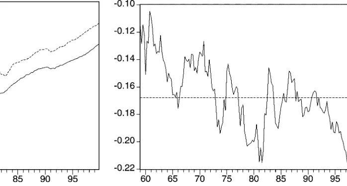
The differences in the average growth rates in the consump-tion and income series in recessions and expansions may have consequences for analyzing the permanent income hypothesis. A simple cointegration analysis in a linear (vector) autoregres-sive model (e.g., Jin 1995) may lead to the wrong conclusion. If the growth rates in both series are different in both stages of the business cycle, then it is unlikely that a linear combination of the two series has a constant mean. To make this more clear, Figure 2 depicts the difference between log per capita consump-tion and log per capita income. The graph shows that the mean of this possible cointegration relation is not constant over time, but rather displays a more-or-less changing regime pattern. This switching pattern seems to coincide with the NBER-dened business cycle.
Relating the stylized facts to the simple model in Section 2, we note that the possible changes in the mean of the differ-ence between log consumption and income are captured by the switching constant·0C·1st in (9). But the differences in growth rates of both series in each stage of the business cycle are not captured by the model, because relation (11) implies that the growth rates in both series during recessions and expansions must be the same. A consumption–income relation that allows for the former behavior is given by
lnctD·0C·1stC¯2lnyt: (12)
The trend in consumption now equals ¯2nt, where nt is the Markov trend in log income dened in (6). If ¯2<1, ·0>0, and·0C·1<0, then the growth rate is smaller in consump-tion than in income during expansions and larger during reces-sions, which corresponds to our earlier ndings. We note that relation (12) corresponds to a nonlinear relation between con-sumption and income, that is,ctDe·0C·1sty¯t2.
To analyze the permanent income hypothesis for the U.S. consumption and income series, we propose a multivariate Markov trend model in the next section. This multivariate model is an extension of Hamilton’s univariate model. The
Figure 2. Difference Between Log Per Capita Consumption and Log Per Capita Income, 1959.1–1999.4.
model contains a multivariate Markov trend that allows for dif-ferent growth rates in the consumption and income series dur-ing recessions and expansions. The deviations from the Markov trend are modeled by a VAR model. To analyze the presence of a consumption–income relation, we perform a cointegration analysis on the deviations from the multivariate Markov trend. In addition, we investigate whether the mean of the possible cointegration relation is affected by changes in the business cy-cle, as suggested by the economic theory in Section 2.
4. THE MULTIVARIATE MARKOV TREND MODEL
In this section we propose the multivariate Markov trend model on which we base our analysis of the consumption– income relation. This model is a multivariate generalization of the model proposed by Hamilton (1989), where the slope of the multivariate Markov trend is different across series and across the regimes. The regime changes occur simultaneously in all series. The deviations from the Markov trend are modeled by a VAR model, which may contain unit roots. A similar represen-tation was suggested by Dwyer and Potter (1996).
In Section 4.1 we discuss representation, and in Section 4.2 we deal with model interpretation. In Section 4.3 we derive the likelihood function of the model. Although we explain the model for bivariate time series, the discussion can be easily ex-tended to more than two time series, as shown in Section 9.
4.1 Representation
LetfYtgTtD1denote a two-dimensional time series containing the log of per capita consumption and income series. Assume thatYtD.lnct lnyt/0can be decomposed as
YtDNtCRtCZt; (13)
whereNt represents a trend component,Rt allows for possible level shifts, and Zt represents the deviations fromNt and Rt. The two-dimensional trend componentNtis a multivariate gen-eralization of the univariate Markov trend (6), that is,
NtDNt¡1C00C01st; (14)
where 00 and 01 are .2£1/parameter vectors and st is an unobserved rst-order Markov process with transition proba-bilities given in (7). Kim and Yoo (1995) added an extra nor-mally distributed error term to (14), but we do not pursue this here, because it a priori imposes a unit root in the seriesYt(see also Luginbuhl and de Vos 1999). We allow unit roots to en-terYt only throughZt; see also Section 4.2. The value of the unobserved state variablest models the stages of the business cycle. IfstD0 (expansion), then the slope of the Markov trend is00, whereas forstD1 (recession), the slope equals00C01 (see also Hamilton 1989). The values of the slopes of the trends in the individual series in Yt do not have to be the same even though the changes in the value of the slope occur simultane-ously. The latter assumption can be relaxed (see, e.g., Phillips 1991), but this extension is not necessary for the application in this article. The expected slope value of the Markov trend equals00C01.1¡p/=.2¡p¡q/(see Hamilton 1989). Hence
one may have different slopes values in each regime but the same expected slope. The backward solution of (14) equals
NtD00.t¡1/C01 t
X
iD2
siCN1; (15)
whereN1denotes the initial value of the Markov trend, which is independent oft. Hence the Markov trend consists of a deter-ministic trend with slope00and a stochastic trendPtiD2siwith impact vector01.
The componentRt models possible level shifts in the rst series ofYtduring recessions,
RtD
³
±1 0
´
stD±st; (16)
such that± D.±1 0/0. This term takes care of level shifts in the consumption series during recessions, as suggested by the theory in Section 2. (See Krolzig 1997, chap. 13, for a similar discussion about the role of this term.) The parameter±1turns out to be related to the·1parameter in (9), as discussed at the end of Section 4.2.
The deviations from the Markov trend andRt (i.e.,Zt) are assumed to be a VAR process of orderk[VAR(k)],
ZtD k
X
iD1
8iZt¡iC"t (17)
or, using the lag polynomial notation,
8.L/ZtD.I¡81L¡ ¢ ¢ ¢ ¡8kLk/ZtD"t; (18)
where "t is a two-dimensional vector normally distributed process with mean 0 and a.2£2/positive-denite symmet-ric covariance matrix6, and where8i,iD1; : : : ;k, are.2£2/ parameter matrices.
4.2 Model Interpretation
For our analysis of a potentially stationary relation between log consumption and income, it is convenient to write (17) in error-correction form,
1ZtD5Zt¡1C k¡1
X
jD1
N
8j1Zt¡jC"t; (19)
where 5DPk
jD18j¡I and 8Ni D ¡PkjDiC18j, iD1; : : : ;
k¡1. The characteristic equation of theZtprocess is given by
I¡81z¡ ¢ ¢ ¢ ¡8kzk
D0: (20)
We can now distinguish three cases depending on the num-ber of unit root solutions of the characteristic equation (20). The rst case corresponds to the situation where the solutions of (20) are outside the unit circle. The processZt is station-ary, and henceYt is a stationary process around a multivariate Markov trend. This is in fact the multivariate extension of the model proposed by Lam (1990). We can write
.1Yt¡00¡01st¡±1st/
D5
Á
Yt¡1¡00.t¡2/¡01 t¡1
X
iD2
si¡N1¡±st¡1
!
C
k¡1
X
iD1
N
8i.1Yt¡i¡00¡01st¡i¡±1st¡i/C"t; (21)
where5a full-rank matrix. The vectors00 and00C01 con-tain the slopes of the trend inYt during expansions and reces-sions. The initial value of the Markov trendN1is unknown and plays the role of an intercept parameter vector. The±1parameter models a level shift in the intercept of the Markov trend during recessions for the log consumption series. If stD0, then the initial value of the Markov trend equalsN1, whereas forstD1, this value equalsN1C±st.
The second case concerns the situation of two unit root solu-tions of (20) with the remaining roots outside the unit circle. In that case,5D0, and (21) becomes
.1Yt¡00¡01st¡±1st/
D
k¡1
X
iD1
N
8i.1Yt¡i¡00¡01st¡i¡±1st¡i/C"t: (22)
The rst difference of Yt is a stationary VAR process with a stochastically changing mean (D00C01st). Note that the ini-tial value of the Markov trend N1 drops out of the model. If
stDst¡1, then1Ytis not affected byRt. If, however,st6Dst¡1, then the growth rate in consumption is±1larger or smaller than the growth rate in income. A change in the stage of the business cycle leads to a one-time extra adjustment in the growth rate of per capita consumption. This adjustment is absent if±1D0, in which case the model simplies to the one considered by Kim and Nelson (1999a), who a priori imposed that5D0 (see also Hamilton and Perez-Quiros 1996).
The third case corresponds to the situation where only one of the roots equals unity and the other roots are outside the unit circle. The series inZtare said to be cointegrated (see Johansen 1995 for a discussion on cointegration). Under cointegration, the rank of5 equals 1, and we can write5 as®¯0, where® and¯ are.2£1/vectors. The¯ vector describes the cointe-gration relation between the elements ofZt, and hence¯0Ztis a stationary process. The® vector contains the adjustment pa-rameters. Because the number of free parameters in®and¯is larger than in5under rank reduction, the parameters in®or¯ must be restricted to become estimable. We choose to impose the restriction¯D.1 ¡¯2/0. Under cointegration, model (21) becomes
.1Yt¡00¡01st¡±1st/
D®¯0
Á
Yt¡1¡00.t¡2/¡01 t¡1
X
iD2
si¡N1¡±st
!
C
k¡1
X
iD1
N
8i.1Yt¡i¡00¡01st¡i¡±1st¡i/C"t: (23)
The cointegration relation is given by¯0YtD¯0.NtCRtCZt/. For ¯000D¯001D0, ·0D¯0N1, and ·1 D¯0±, we obtain the consumption–income relation (12). The extra condition ¯2D1 leads to relation (9). Finally, note that the restriction
¯001D0 removes the Markov trend from the cointegration re-lation. Dwyer and Potter (1996) refered to this phenomenon as “reduced-rank Markov trend cointegration.” Note that in their model,±1D0.
4.3 The Likelihood Function
To analyze the multivariate Markov trend model, we derive the likelihood function. First, we consider the likelihood
func-tion of the least-restricted Markov trend stafunc-tionary model [(21)] conditional on the statesst. The conditional density of Yt for this model, given the past and current states stD fs1; : : : ;stg and given the past observationsYt¡1D fY1; : : : ;Yt¡1g, is
f.YtjYt¡1;st; 00; 01;N1; ±1; 6; 5;8/N
D 1
.p2¼ /2j6j ¡1
2exp
³
¡1
2" 0 t6¡1"t
´
; (24)
where "t is given in (21) and8N D f N81; : : : ;8Nk¡1g. Hence the likelihood function for model (21), conditional on the statessT and the rstkinitial observationsYk, is
L 2.YTjYk;sT; 22/DpN0;0.1¡p/N0;1qN1;1.1¡q/N1;0
£
T
Y
tDkC1
f.YtjYt¡1;st; 00; 01;N1; 6; 5;8/;N (25)
where22D f00; 01;N1; ±1; 6; 5;8;N p;qgand whereN i;j de-notes the number of transitions from stateito statej. The un-conditional likelihood functionL 2.YTjYk; 22/can be obtained by summing over all possible realizations ofsT,
L 2.YTjYk; 22/D
X
s1
X
s2
¢ ¢ ¢X
sT
L 2.YTjYk;sT; 22/: (26)
The unconditional likelihood function for the Markov trend model with one cointegration relation [(23)] follows directly from (26),
L 1.YTjYk; 21/DL 2.YTjYk; 22/j5D®¯0; (27)
with 21 D f00; 01;N1; ±1; 6; ®; ¯2;8;N p;qg. In case of no cointegration [(22)], the unconditional likelihood function is given by
L 0.YTjYk; 20/DL 2.YTjYk; 22/j5D0; (28)
with 20D f00; 01;N1; ±1; 6;8;N p;qg. Note that the subscript “r” of2randL rrefers to the number of cointegration relations inZt.
In the next section we discuss the prior distributions for the model parameters of the multivariate Markov trend model pre-sented in this section.
5. PRIOR SPECIFICATION
To perform inference on the parameters of the multivariate Markov trend model and on the presence of a stationary rela-tion between consumprela-tion and income, we opted for a Bayesian approach. We chose to impose prior information, which is rela-tively uninformative compared with the information in the like-lihood. The Markov trend model is nonlinear in certain para-meters, which leads to local nonidentication for certain pa-rameters in the model. In sum, we must deal with three types of identication issues: the initial value identication (N1), the regime identication (00 and01) and the identication of¯2 in the reduced-rank model (23). To tackle these identication problems, we proceed as follows.
It follows from (21) that the parameterN1 drops out of the model in case5D0. Even in the case of rank reduction in5 it follows from (23) that we can identify only ¯N1. Specify-ing a diffuse prior onN1implies that the conditional posterior
ofN1given5is constant and nonzero at the point of rank re-duction. The integral over this conditional posterior at the point of rank reduction is, therefore, innity, favoring rank reduction (see Schotman and van Dijk 1991a,b for a related discussion of identication problems associated with the intercept term in univariate autoregressions). To circumvent this identication problem, we follow the prior specication of Zivot (1994) (see also Hoek 1997, chap. 2). The prior distribution forN1 condi-tional on both 6 and the rst observationY1 is normal with meanY1and covariance6,
N1jY1; 6»N.Y1; 6/: (29)
For6, we take a standard inverted Wishart prior with scale pa-rameterSand degrees of freedomº,
p.6// jSj21ºj6j¡12.ºC3/exp
³
¡1
26 ¡1
2S
´
: (30)
If we do not want to impose an informative prior for6, then we opt forp.6// j6j¡1, which results from (30) by letting the degrees of freedom approach 0 (see Geisser 1965).
The prior distributions for the transition probabilitiespandq are independent and uniform on the unit interval.0;1/,
p.p/DI.0;1/;
(31) p.q/DI.0;1/;
where I.0;1/ represents an indicator function that is 1 on the
interval (0,1) and 0 elsewhere. Under at priors for p andq, special attention must be given to the priors for 00and01. It is easy to show that under5D0, the likelihood has the same value if we switch the role of the states and change the values of 00,01,±,p, andqinto00C01,¡01,¡±,q, andp. This com-plicates proper posterior analysis if we specify uninformative priors on00and01. There are several ways of identifying the parameters. One could, for example, specify appropriate matrix normal prior distributions for 00 and01. But we dene pri-ors for 00 and01 on subspaces that identify the regimes for all specications of the model. Several specications for these subspaces are possible. With our present application in mind, we restrict the growth rates in the income series to be positive during expansions and negative in recessions. This results in the prior specication
p.00//
»
1 if002 f002R2j00;2>0g 0 elsewhere,
(32)
p.01j00//
»
1 if012 f012R2j00;2C01;2·0g 0 elsewhere.
Note that because we have identied the two regimes by the prior on00and01, we may use an improper prior for±1,
p.±1//1: (33)
For the autoregressive parameters apart from5, we also use at priors,
p.8Ni//1; iD1; : : : ;k¡1: (34)
The three model specications are different with respect to the rank of 5. Under cointegration, the rank of 5 equals 1, and we can write5D®¯0. It is easy to see that if®D0, then
¯2 is not identied (see Kleibergen and van Dijk 1994 for a general discussion). To solve this identication problem, we follow the approach of Kleibergen and Paap (2002) (see also Kleibergen and van Dijk 1998 for a similar approach in simul-taneous equation models). A convenient byproduct of this ap-proach is a Bayesian posterior odds analysis for the rank of5; see also Section 7. The analysis is based on the following de-composition of the matrix5:
5D®¯0C®?¸¯?0 ; (35)
where®?and¯?are specied such that®?0 ®D0 with®0?®?D 1 and¯?0¯ D0 with¯?0 ¯?D1. It is easy to see that cointe-gration (i.e., rank reduction in5) occurs if ¸D0, and hence the parameter¸can be used to test for cointegration. The ma-trix.®?¸¯?0 /models the deviation from cointegration.The row and column spaces of this matrix are spanned by the orthogo-nal complements of the vector of adjustment parameters®and the cointegrating vector¯. The decomposition in (35) is not unique, however. To identify®and¯, we impose the condition that¯D.1 ¡¯2/0, as is often done in cointegration analysis. To identify¸,®?, and¯?in®?¸¯?0 , we relate¸to the small-est singular value of5. Note that singular values determine the rank of5in an unambiguous way.
The singular value decomposition of5is given by
5DUSV0; (36)
whereU andV are.2£2/orthonormal matrices and Sis an .2£2/ diagonal matrix containing the positive singular val-ues of5(in decreasing order) (see Golub and van Loan 1989, p. 70). If we write
UD
³
u11 u12
u21 u22
´
; SD
³
s11 0 0 s22
´
; and
(37)
VD
³
v11 v12
v21 v22
´
;
withuij;sij,vij,iD1;2,jD1;2, scalars and use that
.® ®?/
³
1 0 0 ¸
´
.¯0¯?0 /DUSV0; (38)
then we obtain the following expressions for®and¯2:
®D
³
u11s11v11
u21s11v11
´
(39) ¯2D ¡v21=v11:
Identication of¸follows from the fact that we must express ®?and¯?in terms ofu11,u21,s11,v11andv21to obtain a one-to-one relation with the singular value decomposition. Kleiber-gen and Paap (2002) showed that if we take
®?D
q
u222
³
u12u¡221 1
´
and ¯?D
q
v222
³
v¡221v12 1
´
;
(40) then¸is identied by
¸Dqu22s22v22
u222
q
v222
Dsign.u22v22/s22; (41)
where “sign.¢/” denotes the sign of the argument. Hence the absolute value of¸is equal to the smallest singular value of5 that corresponds tos22. Note that ¸can be positive and neg-ative, in contrast with the singular values22, which is always positive. Golub and van Loan (1989) showed that the number of nonzero eigenvalues of a matrix completely determine the rank of a matrix. Restricting the scalar¸to equal 0 is, therefore, an unambiguous way of restricting the rank of5and imposing cointegration.
To construct priors for the®and¯2parameters that take into account the identication problem, we take as starting point the prior for5given6, denoted byp.5j6/. Because the matrix5 can be decomposed using (35),p.5j6/ implies the following joint prior for®,¸, and¯2given6:
p.®; ¸; ¯2j6//p.5j6/j5D®¯0C®?¸¯0
?jJ.®; ¸; ¯2/j; (42)
wherejJ.®; ¸; ¯2/jis the Jacobian of the transformation from
5to.®; ¸; ¯2/. The derivation and expression of this Jacobian are given in Appendix A. Because restricting¸ to equal 0 is an unambiguous way of restricting the rank of5 and impos-ing cointegration, we construct the joint prior for®and¯2by restricting (42) in¸D0,
p.®; ¯2j6//p.®; ¸; ¯2j6/j¸D0
/p.5j6/j5D®¯0jJ.®; ¸; ¯2/j¸D0: (43)
The posterior resulting from this prior leads to proper posterior distributions for®and¯2(see Kleibergen and Paap 2002). The posteriors are also unique in the sense that they do not depend on the ordering of the variables in the system and the normal-ization to identify® and¯ [in our case,¯D.1 ¡¯2/0]. The proposed strategy for prior construction for® and¯2 can be carried out for a proper or an improper prior specication on5 given6. In this article we opt for a normal prior on5given6 with meanPand covariance matrix.6A¡1/,
p.5j6// j6j¡1jAjexp
³
¡1
2tr
¡
6¡1.5¡P/0A.5¡P/¢
´
:
(44) Hence the prior for®and¯2is given by
p.®; ¯2j6/
/ j6j¡1jAjexp
³
¡1
2tr
¡
6¡1.®¯0¡P/0A.®¯0¡P/¢ ´
£j J.®; ¸; ¯2/j¸D0: (45)
If one prefers a noninformative prior, then one may consider p.5j6//1 in combination withp.6// j6j¡1. In that case, the resulting prior for ® and ¯2, given 6, is p.®; ¯2j6/ /
jJ.®; ¸; ¯2/j¸D0.
The joint priors for the Markov trend models with differ-ent numbers of unit roots follow from the marginal priors in this section. The joint prior for the Markov trend stationary model [(21)], p2.22/, is given by the product of (29)–(34) and (44). The prior for the Markov trend model with one coin-tegration relation [(23)], p1.21/, is the product of (29)–(34) and (45), whereas the prior for the model without cointegra-tion [(22)],p0.20/, is simply the product of (29)–(34).
6. POSTERIOR DISTRIBUTIONS
The posterior distributions for the model parameters of the multivariate Markov trend models is proportional to the prod-uct of the priors,pr.2r/, and the unconditionallikelihood func-tions,L r.YTjYk; 2
r/,rD0;1;2. These posterior distributions are too complicated to enable the analytical derivation of pos-terior results. As Albert and Chib (1993), McCulloch and Tsay (1994), Chib (1996), and Kim and Nelson (1999b) have demon-strated, the Gibbs sampling algorithm of Geman and Geman (1984) is a very useful tool for the computation of posterior results for models with unobserved states. The state variables
fstgTtD1 can be treated as unknown parameters and simulated alongside the model parameters. This technique is known as data augmentation(see Tanner and Wong 1987).
The Gibbs sampler is an iterative algorithm in which one con-secutively samples from the full conditional posterior distribu-tions of the model parameters. This produces a Markov chain that converges under mild conditions. The resulting draws can be considered as a sample from the posterior distribution. (For details on the Gibbs sampling algorithm, see Smith and Roberts 1993; Tierney 1994.) In Appendix B we derive the full condi-tional posterior distributions associated with the most general Markov trend stationary model [(21)]. The full conditionalpos-terior distributions associated with the other models can be de-rived in a similar way. Unfortunately, the full conditionaldistri-butions of the®and the¯2parameters are not of a known type. To sample these parameters we need to build a Metropolis– Hastings step into the Gibbs sampler (see Chib and Greenberg 1995 for a discussion).
7. DETERMINING THE COINTEGRATION RANK
To determine the cointegration rank, we begin by assigning prior probabilities to every possible rank of5
Pr[rankDr]; rD0;1;2: (46)
This is equivalent to assigning prior probabilitiesto the different possible number of cointegration relations,r. The prior proba-bilities imply the following prior odds ratios (PRORs):
PROR.rj2/D Pr[rankDr]
Pr[rankD2]; rD0;1;2: (47)
The Bayes factor (BF) for comparing rankrwith rank 2 equals
BF.rj2/D
R
L r.YTjYk; 2r/pr.2r/d2r
R
L 2.YTjYk; 2
2/p2.22/d22
; rD0;1; (48)
where L r.YTjYk; 2
r/ denotes the unconditional likelihood function and pr.2r/denotes the joint prior of the model with rankr. The posterior odds ratio (POR) for comparing rank r with rank 2 equals the PROR times the BF, POR.rj2/D PROR.rj2/£BF.rj2/, and the posterior probabilities for each rank are simply
Pr[rankDrjYT]D POR.rjn/
P2
iD0POR.ij2/
; rD0;1;2: (49)
The BFs in (48) are in fact BFs for5D0 and¸D0. They can be computed using the Savage–Dickey density ratio of Dickey (1971), which states that the BF for5D0 (or¸D0)
equals the ratio of the marginal posterior density and the mar-ginal prior density of5(¸), both evaluated in5D0 (¸D0),
BF.0j2/Dp.5jY
T/j
5D0
p.5/j5D0
;
(50)
BF.1j2/Dp.¸jY
T/j
¸D0
p.¸/j¸D0
:
This means that we need the marginal posterior densities of 5 and¸ to compute these Savage–Dickey density ratios. The marginal posterior density of5can be computed directly from the Gibbs output by averaging the full conditional posterior dis-tribution of5 in the point 0 over the sampled model parame-ters (see Gelfand and Smith 1990). This approach cannot be used for¸, because the full conditional distribution of¸ is of an unknown type. To compute the height of the marginal pos-terior of¸, we may use a kernel estimator on simulated¸ val-ues (see, e.g., Silverman 1986). Another possibility is to use an approximation of the full conditional posterior of¸in combi-nation with importance weights (see Chen 1994). Kleibergen and Paap (2002) argued that the density functiong.¸j21;YT/ dened in (B.13) is a good approximation. This results in the following expression to compute the marginal posterior height at¸D0:
p.¸jYT/j¸D0¼ 1 N
N
X
iD1
jJ.®i; ¸; ¯2i/j¸D0j
jJ.®i; ¸i; ¯i 2/j
g.¸j2i1;YT/j¸D0;
(51) whereN denotes the number of simulations. Note that we can avoid the importance weights by using numerical integration to determine the integrating constant of the full posterior condi-tional distribution of¸in every Gibbs step.
Because we have a closed form for the prior density of5, we can compute the prior height of 5 at 5D0 directly. To compute the prior height of ¸, we follow a similar procedure as for the posterior height. First, we sample from the prior of 6 and5, given6. Next, we perform a singular value decom-position on the sampled5i (37), resulting in¸i ®i and¯2i. To compute the marginal prior height of¸at¸D0, we may use a kernel estimator on the sampled¸i. Again, it is possible to use an approximation of the full conditional prior of ¸in combi-nation with importance weights. The prior height can be com-puted as
p.¸/j¸D0¼ 1 N
N
X
iD1
jJ.®i; ¸; ¯2i/j¸D0j
jJ.®i; ¸i; ¯i 2/j
h.¸j2i1/j¸D0; (52)
whereh.¸j21/is an approximation of the full conditional prior distribution of¸. An appropriate candidate forhturns out to be
h.¸j21/D.2¼ /¡
1
2j®?6¡1®0
?j
1 2j¯0
?A¯?j
1 2
£exp
³
¡1
2tr
¡
¯?0A¯?.¸¡l/®?6¡1®?0 .¸¡l/0¢
´
; (53)
withlD.¯?0A¯?/¡1¯?0A.P¡¯ ®/6¡1®0?.®?6¡1®?0 /¡1. Finally, if we species an improper prior for5and¸, then the height of the marginal prior at5D0 and¸D0 is not de-ned. Therefore, the BFs in (50) are not properly dened in cases of diffuse priors. Kleibergen and Paap (2002) argued that
a Bayesian cointegration analysis under a diffuse prior speci-cation on5 is possible if one replaces the prior height by the
factor.2¼ /¡12.2¡r/2. This leads to a BF that corresponds to the
posterior information criterion (PIC) of Phillips and Ploberger (1994). We opt for the same solution in this article.
8. U.S. CONSUMPTION AND INCOME
In this section we analyze the presence of a long-run rela-tion between the U.S. per capita consumprela-tion and income se-ries considered in Section 3. We rst start in Section 8.1 with a simple analysis of cointegration between the two series in a VAR with a linear deterministic trend to illustrate the effects of neglecting the presence of a possible Markov trend in the series. In Section 8.2 we analyze the presence of a long-run re-lation between consumption and income using the multivariate Markov trend model proposed in Section 4.
8.1 A Vector Autoregressive Model Without Markov Trend
If we restrict01and±1in the Markov trend model (21) to 0, then we end up with a VAR forYtwith only a linear determinis-tic trend. In this section we analyze the presence of a cointegra-tion relacointegra-tion between U.S. per capita consumpcointegra-tion and income in this VAR forYtD100£.lnct;lnyt/0. The priors forN1and
6 are given by (29) and (30), withSDI andºD3. For 5, given6, we opt for ag-type prior (see Zellner 1986). This prior is given in (44) withPD0 andAD¿ =TPT
tD1YNt0YNt for differ-ent values of¿, whereYNtdenotes the demeaned and detrended value ofYt. Because we are dealing with nonstationary time se-ries, we divide by the number of observations,T (see Kleiber-gen and Paap 2002 for a similar approach). A smaller value of ¿ implies less precision in the prior information on5j6. For 00and8Niwe take at priorsp.00//1 andp.8Ni//1.
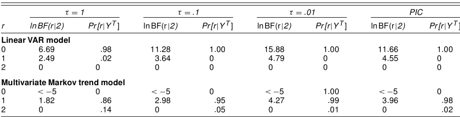
Before beginning our analysis, we must choose the lag order kof the VAR model. To determine the lag order, we sequen-tially test for the signicance of an extra lag using PIC-based Bayes factors starting withkD1. Given this strategy we nd thatkD2. We note that the same lag order is found using the Bayes information criterion (BIC) of Schwarz (1978) to deter-minek. For the cointegration analysis, we assign equal prior probabilities to the possible cointegration ranks (46), that is, Pr[rankDr]D13 forrD0;1;2. The prior for®and¯2for the cointegration specication (rank=1) is given by (45).
Columns 2–7 in the rst panel of Table 1 shows log BFs and posterior probabilities for the cointegration rankrfor different values of¿. The results show that a model with a rank of 5 of 0 or 1 is preferred over a model with full rank for5. The log BFs computed for the model with rank 0 versus the model with rank 1 are 4.20 (6.69–2.49), 7.64, and 11.09 for¿ equal to 1, .1, and .01. Hence the model with no cointegration relation is preferred over the model with 1 cointegration relation. The BFs lead to the assignment of 98% posterior probability to the model with no cointegration relation if¿D1 and 100% for the other values of¿. In sum, there is no evidence for a long-run equilibrium between U.S. per capita consumption and income in a VAR model with only a linear deterministic trend. [The standard trace tests for rank reduction (Johansen 1995) also do
Table 1. Log BFs and Posterior Probabilities for the Cointegration Rank in a Linear VAR Model (kD2) and the Multivariate Markov Trend Model (kD1)
¿D1 ¿D:1 ¿D:01 PIC
NOTE: A log BF, ln BF(rj2)>0, denotes that a cointegration model withrcointegration relations is more likely than a model with two cointegration relations. The posterior probability of the cointegration rank, Pr [rjYT], is dened in (49) and based on equal prior probabilities (46) for every rankr. Posterior results are based on 400,000 iterations with the Gibbs sampler, neglecting the rst 100,000 draws.
not indicate the presence of a cointegration relation between the two series.] Unreported results show that this nding is robust with respect to the chosen lag order. The log BFs for models with order 2<k·5 are very similar to those reported in Ta-ble 1.
The results in Table 1 show that if we increase the prior vari-ance of5 by decreasing¿, then the evidence for rank reduc-tion, and hence the presence of unit roots, increases. This is due to the fact that our prior is centered at 5D0. When we in-crease the prior variance, the prior height at5D0 decreases. The posterior height at 5D0 remains almost the same, be-cause the value of¿ is so small that the prior has only a mini-mal effect on the posterior. From Section 7, we have seen that the BF for5D0 equals the ratio of the posterior and prior heights at5D0, and hence that too small a value of¿ leads to rank reduction being favored, no matter what the nature of the sample evidence. This phenomenon is known as the Lind-ley paradox(see Zellner 1971). In the second-to-last column of the rst panel of Table 1, we report the log BFs for improper priors on5and6, that is, p.5; 6// j6j¡1. Under this prior specication, BFs are not dened properly. Instead, we report a PIC-based BF, where we replace the prior heights in (50) by the
penalty function.2¼ /¡12.2¡r/2. These BFs again indicate that
rank reduction is preferred to the full-rank case and lead to the assignment of 100% posterior probability to the model with no cointegration relation.
With no cointegration imposed, the estimated VAR model is
O
where the point estimates are posterior means based on the im-proper prior specication discussed earlier and posterior stan-dard deviations are given in parentheses. Note that this model is equal to (13)–(17) with01D0,±1D0, andkD1. The poste-rior means of the slopes of the deterministic trends in the con-sumption and income series are .63% and .68%. They differ by about .01% from the average quarterly growth rates reported in Section 3. Note that this difference is small compared with the posterior standard deviations of the slopes.
8.2 A Bivariate Markov Trend Model
The VAR model with a deterministic trend assumes that the quarterly growth rates of consumption and income are constant over time. However, the stylized facts suggest that the long-run average quarterly growth rates are roughly the same, but there may be different growth rates in both series during ex-pansions and recessions. To allow for the possibility of differ-ent growth rates in consumption and income during recessions and expansions, we consider the Markov trend model (21). The prior for the model parameters is given by (29)–(34) withSDI andºD3. For5given6, we again use the sameg-type prior as for the non-Markov model. The prior is given in (44) with PD0 andAD¿=TPT
tD1YNt0YNt, whereYNt denotes the demeaned and detrended value ofYt.
Again, we perform a cointegration analysis, but now we an-alyze, the presence of a cointegration relation in the deviations from a Markov trend instead of a deterministic trend. To deter-mine the lag order of the VAR part of the model, we use the same strategy as for the non-Markov model. It turns out that one lag is sufcient, and hence we impose kD1. We assign equal probabilities to the possible cointegration ranks, that is, Pr[rankDr]D13 forrD0;1;2. The prior for®and¯2for the cointegration specication (rD1) is given by (45). Columns 2–7 of the second panel of Table 1 report the log BFs and pos-terior probabilities for the rank of5for different values of¿. Comparing the corresponding results in the rst panel, where we show the results for the model without Markov trend, we see that all log BFs are smaller. Not surprisingly, there is more posterior evidence for rank reduction if we allow for a Markov trend instead of a deterministic trend. For all values of¿, the model with two unit roots (rD0/is clearly rejected against both the cointegration (rD1/and the Markov trend stationary (rD2/specications. The posterior probabilities assign more
than 86% posterior probability to the cointegration specica-tion. For¿D:01, we nd the least evidence for cointegration, although the evidence is certainly not weak. As discussed ear-lier, under this prior specication we a priori favor the presence of two unit roots and no cointegration, because the prior height at5D0 in the second BF in (50) is relatively small. The -nal two columns of the second panel of Table 1 refer to the case where we impose an improper prior on5and6. We re-port again a PIC-based log BF, where replace the prior heights in (50) by the penalty function.2¼ /¡12.2¡r/2. The log BFs
im-ply an assignment of 98% posterior probability to the cointe-gration specication.
Overall, the BF analysis suggests that the multivariate Markov trend model with one cointegration relation [(23)] is suitable for modeling the logarithm of U.S. per capita consump-tion and income. The estimated model is given by
O
where the point estimates are posterior means and posterior standard deviations appear in parentheses. Because the poste-rior distribution of¯2 may have Cauchy-type tails, we report the posterior mode. (This is also done for other posterior quan-tities involving¯2.) The posterior means of the transition prob-abilities equal
O
pD:86.:05/ and qOD:76.:10/:
The posterior results are based on the prior specication (29), (31)–(34), p.6// j6j¡1, and p.®; ¯2j6/ / jJ.®; ¸; ¯2/j¸D0 and are obtained by including a Metropolis–Hastings step in the Gibbs sampler to sample® and¯2; see Appendix B. The candidate draw for ® and ¯2 was accepted in about 70% of the iterations. Note that a noninformative prior does not lead to problems if one just wants to estimate the model parameters without testing the rank.
Figure 3 shows the posterior density of ¯2. The posterior mode of the cointegration relation parameter is¡:81. The 95% highest posterior density (HPD) region for¯2is.¡1:05;¡:65/, and hence¡1 is included just in this region. There is only weak evidence for the consumption–income relation (9). The adjustment parameters:24 and:55 are both positive, which in-dicates that there is no adjustment toward equilibrium for the consumption equation. Note that this does not imply that the
Figure 3. Posterior Density of¯2.
series move away from the equilibrium, because the adjustment of income toward equilibrium is larger than the nonadjustment in consumption (see also Johansen 1995, pp. 39–42).
The posterior mean of the±1parameter equals .15. The 95% HPD region for this parameter is.¡:31; :59/, and hence it is very likely that±1equals 0. The posterior means of the quar-terly growth rates of the income series are 1:16% during an expansion regime and¡:17% (1.16–1.33) during a contraction regime. For the consumption series, we get .83% and :23% (.83–.60). Hence during recessions, the growth rate in con-sumption is larger than the negative growth rate in income. To correct for this difference in the growth rates, the growth rate in income has to be larger than the growth rate in consumption during expansions.
Reduced-rank Markov trend cointegration (¯001D0) is not likely, because the posterior mode of¯001 equals:44 and its 95% HPD region is.:20; :89/. The 95% HPD region of¯000 is.¡:39; :37/with a posterior mode of¡:08. Hence the exis-tence of a consumption–income relation (9) requiring that both ¯001and¯000equal 0 is not likely. On the other hand, the re-sults suggest that during recession periods, the growth rate in consumption is larger than in income, which is compensated for in the expansion periods, where income grows faster than consumption.
The expected slope of the Markov trend equals00C01.1¡
p/=.2¡p¡q/(see Hamilton 1989). The posterior mean of the expected slope of the Markov trend is .65% for the income se-ries and .60% for the consumption sese-ries. These values differ by only .02 from the average quarterly growth rates reported in Section 3. The 95% HPD region of the expected slope of the Markov trend in the cointegration relation is.¡:10; :46/, and the posterior mode equals .08. During recessions the posterior mode of the growth of the cointegration relation¯0.00C01/ is :34 .:21; :62/, whereas during expansions it equals ¡:08 .¡:39; :37/as reported before.
Finally, we analyze how the estimated Markov trend relates to the NBER turning points. The posterior mean of the proba-bility of staying in the expansion regime is .86, which is larger than the posterior mean of the probability of staying in a re-cession, .76. The posterior probability thatp is larger than q
Figure 4. Posterior Expectations of the State VariablesE[stjYT].
is .88, which indicates the existence of an asymmetric cycle. Figure 4 shows the posterior expectationsof the states variables, E[stjYT]. Values of these expectation close to 1 correspond to recessionary periods. Figure 5 shows the difference between the logarithm of U.S. income and consumption. The shaded areas correspond to the recessionary periods, where the growth rate in consumption is larger than the growth rate in income.
Table 2 indicates the estimated peaks and troughs based on the posterior expectation of the states variables together with the ofcial NBER peaks and troughs. We dene a recession by two consecutive quarters for which E[stjYT]> :5. A peak is dened by the last expansion observation before a recession; a trough, by the last observation in a recession. We see that the estimated turning points correspond very well with the ofcial NBER peaks and troughs. However, we detect two extra reces-sionary periods that do not correspond with ofcial reported recessions. Remember that the consumption income analysis in this article is based on per capita disposable income. Look-ing at the government purchases on goods and services used to create the disposable income series, we see that government
Figure 5. Difference Between Log U.S. Per Capita Consumption and Income. The shaded areas correspond to recessionary periods.
Table 2. Peaks and Troughs Based on the Posterior Expectations of the Unobserved
State Variables
U.S. NBER
Peak Trough Peak Trough
1960.1 1960.4 1960.2 1961.1 1966.1 1967.4
1968.2 1970.4 1969.4 1970.4 1973.2 1975.1 1973.4 1975.1 1979.3 1980.2 1980.1 1980.3 1981.3 1982.4 1981.3 1982.4 1984.4 1987.3
1989.2 1991.1 1990.3 1991.1
NOTE: A recession is dened by two consecutive quarters for which E[stjY T]> :5. A peak corresponds with the last expansion observation before a recession, a trough, with the last observation in a recession.
expenses increase during recessions, resulting in an extra de-crease in disposable income. However, there was also a large increase in government expenses during the two periods incor-rectly reported as recessions. This resulted in a small decline or a smaller growth in disposable income during these two peri-ods, which explains the detection of the two extra recessions in our data.
In summary, the multivariate Markov trend model provides a good description for the U.S. per capita income and consump-tion series. The multivariate Markov trend captures the differ-ent growth rates in both series during recession and expansion periods. After detrending with the Markov trend, we detect a stationary linear combination between log per capita income and consumption. This cointegration relation is not found if we use a regular deterministic trend instead of a Markov trend for detrending.
9. U.S. CONSUMPTION, INCOME, AND INVESTMENT
In the previous section we showed the existence of a cointe-gration relation between log per capita income and consump-tion only if a Markov trend is allowed for. We may investigate whether the inclusion of a third variable with a more pro-nounced cyclical pattern can help improve the model. There-fore, in this section we consider a multivariate Markov trend model for per capita real disposable income, private consump-tion, and private investment in the U.S., 1959.1–1999.4. The consumption and income series are the same as in the previous section. The investment series was also obtained from the Fed-eral Reserve Bank of St. Louis. Figure 6 shows a plot of the log of the three series. The investment series clearly demonstrates a more pronounced cyclical pattern than the other two series.
To describe the three series, in Section 9.1 we consider a VAR model without a Markov trend. In Section 9.2 we intro-duce the multivariate Markov trend in the model, where we al-low the growth rates in the three series to be different across the series and across the stages of the business cycle.
9.1 A Vector Autoregressive Model Without Markov Trend
In this section we analyze the presence of a cointegration relations in a VAR model without Markov trend [01D0 and
Figure 6. Logarithm of U.S. Per Capita Consumption (——-), In-come (¢ ¢ ¢ ¢), and Investment (- - - -), 1959.1–1999.4.
±1D0 in (21)] for YtD100£.lnct;lnyt;lnit/0, where it de-notes per capita investment series. The priors for model para-meters are the same as in the previous example. The priors for N1 and6 are given by (29) and (30), withSDI and ºD4.
The lag order determination is done in the same way as in Section 8. The resulting order is 2, which is also obtained if the BIC is used to determinek. The Bayesian cointegrationanalysis is a multivariate extension of the analysis in Section 7. The prior for®and¯2for the cointegration specications (ranks 1 and 2) are similar to (45). We assign equal prior probabilities to the possible cointegration ranks (46), that is, Pr[rankDr]D14 for rD0;1;2;3.
The rst panel of Table 3 displays the log BFs together with the posterior probabilities for different values of¿. For all val-ues of ¿, the BFs lead to 100% probability of a VAR model with 1 cointegration relation. [The standard Johansen (1995) trace tests do not indicate the presence of a cointegration lation between the three series if the deterministic trend is
re-stricted within the cointegration space.] This is also true if one chooses to consider the PIC-based BFs.
The posterior results suggests that we must consider a VAR(2) model with 1 cointegration relation. The estimated model is given by
where again the point estimates are posterior means (except for the cointegration relation parameters) and posterior standard deviations are given in parentheses. The posterior results are based on a diffuse prior specication. The posterior modes of the cointegration relation parameters are¡:95 for the consump-tion series and .24 for the investment series. The corresponding 95% HPD regions are.¡:47;1:07/and.¡2:19; :04/. Note that the HPD regions are quite large, which is due to the relatively small values of the adjustment parameters.
Table 3. Log BFs and Posterior Probabilities for the Cointegration Rank in a Linear VAR Model (kD2) and the Multivariate Markov Trend Model (kD1)
¿D1 ¿D:1 ¿D:01 PIC
NOTE: A log BF, ln BF.rj3/ >0, denotes that a cointegration model withrcointegration relations is more likely than a model with three cointegration relations. Posterior results are based on 400,000 iterations with the Gibbs sampler, neglecting the rst 100,000 draws.
The posterior means of the slope parameters of the consump-tion and income series are somewhat larger than for the bivari-ate model discussed in Section 8.1. The posterior mean of the slope parameter of the investment series corresponds reason-ably well with the average quarterly growth rate of the series equal to .89%.
9.2 A Multivariate Markov Trend Model
To allow for the possibility of different growth rates across the series and across the stages of the business cycle, we con-sider the Markov trend model (21). We take similar prior distri-butions as for the bivariate model in Section 8.2. Hence the prior distributions for the model parameters are given by (29)–(44) withSDI,º D4, PD0, andAD¿=TPT
tD1YNt0YNt, where YNt denotes the demeaned and detrended value ofYt.
The lag order selection procedure for the VAR part of the model results inkD1. The priors for® and¯2for the coin-tegration specications are similar to (45). We again assign equal probabilities to the possible cointegration ranks, that is, Pr[rankDr]D14forrD0;1;2;3. The second panel of Table 3 reports the log BFs and posterior probabilities for the rank of5 for different values of¿. The values of the log BFs are similar to the values in the rst panel of the table. Hence adding a Markov trend to the model does not change the posterior probabilities concerning the number of cointegration relations.
The selected model by the BF is a VAR(1) model with one cointegration relation. The estimated model is given by
O
where again the point estimates are posterior means and poste-rior standard deviations are given in parentheses. The posteposte-rior results are based on a diffuse prior specication. The posterior means of the transition probabilities equal
O
pD:86.:05/ and qOD:76.:10/;
which are equal to those of the bivariate Markov trend model in Section 8.2.
The posterior modes of the cointegration relation parameters are ¡:71 for the consumption series and¡:06 for the invest-ment series. The correspondingHPD regions are.¡1:00;¡:35/ and.¡:18; :06/, which are clearly smaller than those for the linear VAR specication. The adjustment parameters are more than two posterior standard deviations away from 0, and hence the cointegration relation seems more relevant than in the model without the Markov trend. The HPD region of the cointegration relation parameter for investment contains 0, suggesting that any contribution of investment to the cointegration relation is of minor importance.
The posterior means of the Markov trend parameters of the consumption and income series are almost the same as those for the bivariate model in Section 8.1. For the investment se-ries, the posterior mean of the quarterly growth rate is 2.80% during expansions and¡2:32% during recessions (2.80–5.12). Reduced-rank Markov trend cointegration (¯001D0) is again not very likely, because the posterior mode of¯001equals:45, and its 95% HPD region is.:19; :99/.
In sum, we have seen that BFs suggest one out of three pos-sible cointegration relations in a VAR model with deterministic trend for per capita consumption, income, and investment. This implies that there are still two unit roots remaining in the sys-tem, as was also the case in our bivariate specication in Sec-tion 8. Although BFs suggest the presence of one cointegraSec-tion relation, the relevance of the error correction term is small. If we turn to a multivariate Markov trend model, then the error correc-tion term becomes more relevant, and the contribucorrec-tionof invest-ment to the cointegration relation is negligible. The inclusion of a Markov trend now does not lead to a decrease in the number of unit roots in the system as in the bivariate case. Although in-vestment seems to partly replace the role of the Markov trend in the linear VAR, the posterior results of the Markov trend model role suggest that the Markov trend remains important.
10. CONCLUSION
In this article we have proposed using a multivariate Markov trend model to analyze the possible existence of a long-run re-lation between U.S. per capita consumption and income. The model specication was based on suggestions by simple eco-nomic theory and a simple stylized facts analysis on both se-ries. The model contains a multivariate Markov trend speci-cation that allows for different growth rates in the series and different growth rates during recessions and expansions. The deviations from the multivariate Markov trend are modeled by a VAR model. We have chosen a Bayesian approach to analyze U.S. series with the multivariate Markov trend model. BFs are proposed to analyze the presence of a cointegration relation in the deviations of the series from the multivariate Markov trend. The posterior results suggest that there a stationary linear re-lation exists between log per capita consumption and income after correcting for a Markov trend. The Markov trend mod-els the different growth rates in both series during recessions and expansions. The growth rate in consumption is larger than the negative growth rate in income during recessions. To com-pensate for this difference, the growth rate in income is larger
![Figure 4. Posterior Expectations of the State Variables E[stjYT ].](https://thumb-ap.123doks.com/thumbv2/123dok/1156093.766576/12.584.356.518.94.201/figure-posterior-expectations-state-variables-e-stjyt.webp)