Manajemen | Fakultas Ekonomi Universitas Maritim Raja Ali Haji 073500103288619043

(1)

Full Terms & Conditions of access and use can be found at

http://www.tandfonline.com/action/journalInformation?journalCode=ubes20

Download by: [Universitas Maritim Raja Ali Haji] Date: 13 January 2016, At: 01:03

Journal of Business & Economic Statistics

ISSN: 0735-0015 (Print) 1537-2707 (Online) Journal homepage: http://www.tandfonline.com/loi/ubes20

Recent Two-Stage Sample Selection Procedures

With an Application to the Gender Wage Gap

Louis N Christofides, Qi Li, Zhenjuan Liu & Insik Min

To cite this article: Louis N Christofides, Qi Li, Zhenjuan Liu & Insik Min (2003) Recent Two-Stage Sample Selection Procedures With an Application to the Gender Wage Gap, Journal of Business & Economic Statistics, 21:3, 396-405, DOI: 10.1198/073500103288619043

To link to this article: http://dx.doi.org/10.1198/073500103288619043

View supplementary material

Published online: 01 Jan 2012.

Submit your article to this journal

Article views: 78

View related articles

(2)

Recent Two-Stage Sample Selection

Procedures With an Application

to the Gender Wage Gap

Louis N. C

HRISTOFIDES

Department of Economics, University of Cyprus, 1678 Nicosia, Cyprus

Qi L

I

Department of Economics, Texas A&M University, College Station, TX 77843-4228 and School of Economics and Management, Tsinghua University, Beijing, PRC

Zhenjuan L

IU

and Insik M

IN

Department of Economics, Texas A&M University, College Station, TX 77843-4228

Recently developed two-stage estimation methods of sample selection models are used, in the context of data from the 1989 Labor Market Activity Survey, to examine labor supply decisions and wage outcomes for employed men and women. Recent hypothesis test procedures are used to test for no sample selection and to test for a parametric against a semiparametric selection-correction procedure. We conclude that selection is indeed an issue for the sample at hand and that the semiparametric specication is appropriate. We also present the standard decomposition of the gender wage gap into its explained and unexplained portions.

KEY WORDS: Labor supply; Selection; Two-stage semiparametric estimation; Wage outcomes.

1. INTRODUCTION

Empirical work in many areas of economics involves work-ing with subsamples drawn from random samples of the pop-ulation according to specied criteria. For instance, studies of the wage determination process typically involve subsamples of individuals who are employed, work positive hours, and have known wages; the researcher may be interested in the extent to which socioeconomic characteristics may affect wages. The ex-tent to which results based on selected samples can be meaning-ful has been discussed at least as far back as the work by Gronau (1974) and Lewis (1974). Although a number of approaches have been considered, Heckman (1976, 1979) suggested the most widely used procedure: A process describing the employ-ment outcome is impleemploy-mented, and information from this is used in a second stage to obtain consistent estimates of the rele-vant parameters. It is well known that this two-stage procedure can be subject to data-driven problems, including lack of iden-tication and results that are sensitive to specication. (For a careful discussion of this problem in a particular empirical con-text, see Baker, Benjamin, Desaulniers, and Grant 1995. For more recent developments, see Heckman 1990; Manski 1989, 1990; Newey, Powell, and Walker 1990; Vella 1993, 1998.)

Vella (1992) proposed a test for sample selection bias using a type 3 tobit residual as a generated regressor. Using a similar idea, Wooldridge (1994) proposed a two-stage estimator that is simple to use and is more robust than Heckman’s procedure. Wooldridge (1995) further considered the sample selection bias problem with panel data. Wooldridge (1994) also showed that his method can be generalized to allow for nonnormality in the error distributions, a possibility that would render applica-tion of the Heckman (1976, 1979) technique inappropriate. In this case, the model becomes a semiparametric partially linear model with generated regressors entering the model nonpara-metrically. Li and Wooldridge (2002) derived apn-consistent

estimator for this model. Alternative semiparametric, two-stage methods that do not require knowledge of error distributions have been proposed by various authors [e.g., Chen 1997; Hon-ore, Kyriazidou, and Udry 1997 (HKU hereinafter), Lee 1994]. Recently developed consistent model specication tests (e.g., Zheng 1996; Li and Wang 1998) provide the background for hypothesis tests of selection bias and in the event that selection bias is accepted, one can further test for a parametric selection null model versus a semiparametric alternative. Thus a coherent two-stage approach that overcomes some difculties that may arise in the probit-ordinary least squares (OLS) sequence and that tests down from the general (selection vs. no selection) to the particular (parametric vs. semiparametric correction) is now available.

In this article we make extensive and integrated use of these recent developments by considering the problem of estimat-ing labor market involvement and wage equations from sam-ples of employed men and women. Using selection-corrected wage equations, we also consider the gender wage gap and its traditional decomposition into portions explainable by charac-teristics and possible discrimination. We rely on the very large samples that can be drawn from the 1989 Labour Market Activ-ity Survey for Canada, a source for earlier studies of the wage determination process that use the Heckman (1976, 1979) ap-proach.

In Section 2 we briey discuss some recent semiparametric estimation methods for the type 3 tobit model. These will pro-vide the econometric background required in the applied analy-sis. In Section 3 we describe the data, and in Section 4 we pro-vide labour supply and wage equations based on the alternative

396

(3)

estimators and conduct the hypothesis tests required to select the appropriate model. We also report the results of decom-posing observed male–female wage differentials into portions attributable to characteristics and possible discrimination. We present some concluding comments in Section 5.

2. ECONOMETRIC PRELIMINARIES

Consider the type 3 tobit model dened by the latent vari-ables

y¤₁_Dx₁¯1Cu1 (1)

and

y¤₂_Dx₂¯2Cu2; (2) where (1) is the selection equation and (2) is the main equa-tion of interest. The dependent variabley¤₂can be observed only when the selection variabley¤₁is positive. Thus we observey1 andy2, that satisfy

y1Dmaxfy¤₁;0g (3) and

y2Dy¤21fy1>0g; (4) where1fAg represents the indicator function of the eventA,y1 andy2 are the observable dependent variables,x1 and x2 are row vectors of exogenous variables with dimensionp1andp2, and¯1and¯2are conformable column vectors of unknown pa-rameters. In the empirical application considered in Section 4,

y1is the working hours of an individual andy2is the logarithm of the hourly wage rate.

Under the selection rule described by (3) and (4), we have that

E.y¤₂_jx1;x2;y¤1>0/Dx2¯2CE.u2ju1>¡x1¯1;x1;x2/: (5) Hence the least squares method of regressingy2onx2is an inconsistent estimator of ¯2 if the second term on the right-side of (5) is nonzero. Under the joint normality assumption of .u1;u2/, Heckman (1976, 1979) proposed a simple two-stage method for estimating type 2 or type 3 tobit models. Heckman’s suggestion was to restore a zero conditional mean in (4), by including an estimate of the selection bias term,

E.u2ju1>¡x1¯1;x1;x2/. Under normality, this term is propor-tional to the inverse Mills ratio (we denote it by¸) and depends only on unknown parameters of (1), which can be estimated by probit or tobit maximum likelihood.

Vella (1992, 1998) and Wooldridge (1994) have suggested alternative two-stage estimation methods that may have bet-ter nite sample properties. Under the assumption that.x₁;x₂/

are independent of .u1;u2/, Vella and Wooldridge noted that E.u2jx;u1;y1>0/DE.u2ju1;y1>0/. If one further assumes thatE.u2ju1/D°1u1, then the selection bias correction term is°1u1. One can estimateu1byuO1Dy1¡x1¯O1, where¯O1is the tobit estimator of¯1. Thus one can useu1, rather than Heck-man’s (1979) inverse Mills ratio, as an additional variable in the conditional expectation. The advantage is that even when

x2and the inverse Mills ratio are near collinearity,u1has more variation thanx₂, thereby making the Vella–Wooldridge estima-tor more stable and thus more efcient (see Wooldridge 2002, p. 573 for a more detailed discussion).

One can also estimate (3) and (4) simultaneously with the maximum likelihood method by assuming the joint normality of.u1;u2/. Compared with the maximum likelihood method, the Vella–Wooldridge two-step method has at least three advan-tages: (1) it is computationallyless costly, (2) it does not require the joint normality of.u1;u2/, assuming only the normality of u1and thatE.u2ju1/is linear inu1, and (3) it is more robust to near collinearity in data.

As noted by Wooldridge (1994), a further advantage of the Vella–Wooldridge approach is that the assumption of normality can be easily relaxed. There is no need to assume that the joint distribution of.u1;u2/is known or to assume thatE.u2ju1/D

Following Robinson (1988) and using the data withy1i>0,

from (6) we get

y₂i¡E.y2iju1i/D[x2i¡E.x2ju1i/]¯2Cv2i: (7)

Li and Wooldridge (2002) suggested a two-step method for estimating¯2:

1. Estimateu1ibyuO1iDy1i¡x1i¯O1, where¯O1is a rst-stage estimator of¯1, say Powell’s (1984) censored least absolute de-viation (CLAD) estimator, dened by

3. Apply a least squares method to estimate¯2based on (7) (e.g., Robinson 1988).

Li and Wooldridge (2002) also established thepnnormality of their estimator for¯2(denoted by¯O2;LW).

Numerous authors have also suggested semiparametric esti-mation of type 3 Tobit models that do not require knowledge of the joint distribution of.u1;u2/(see, e.g., Chen 1997; HKU 1997; Lee 1994). Later we briey discuss some of the estima-tors proposed by these authors.

Chen (1997) observed that under the condition that.u1;u2/ is independent of.x1;x2/,

E.y2jx1;x2;u1>0;x1¯1>0;y1>0/

DE.y₂_ju₁>0;x/_Dx₂¯2C®0; (9) where®0is a constant but®0is not the intercept of the original model, because an intercept is not identied without further as-sumptions. Based on (9), Chen suggested a simple least squares procedure applied to a trimmed subsample to estimate¯2by

O the estimator proposed by Honore and Powell (1994), or the

(4)

398 Journal of Business & Economic Statistics, July 2003

CLAD estimator of Powell (1984). As discussed by Chen, one problem with the estimator given by (10) is that it may trim out too many observations and hence lead to inefcient estima-tion. Chen (1997) further suggested an alternative estimator that trims much fewer data points in nite-sample applications (see eq. 11 of Chen 1997 for details).

HKU (1997) have proposed an alternative approach. To re-lax the normality assumption of Heckman, HKU considered the case in which the underlying errors are symmetrically distrib-uted conditional on the regressors, with arbitrary heteroscedas-ticity permitted. The effect of sample selection in this case is that the errors are no longer symmetrically distributed condi-tional on the sample selection. HKU (1997) noted that if one estimates¯2using observations for which¡x1¯1<u1<x1¯1 (equivalent to 0<y1<2x1¯1), thenu2 is symmetrically dis-tributed around 0 under this conditioning. Hence the following least absolute deviations estimator consistently estimates¯₂:

O Powell’s (1984) censored least absolute deviations estimator dened earlier. HKU (1997) also established the pn normal-ity of their proposed estimator¯O2;HKU.

Under the assumption of independence between errors and regressors, Lee (1994, eq. 2.12) showed that

y2i¡E.y2ju1>¡x1i¯1;x1¯ >x1i¯1/

D[x₂i¡E.x2jx1¯1>x1i¯1/]¯2C²2i; (12)

where ²2i satises E.²2iju1>¡x1i¯1;x1¯ >x1i¯1/D0. Lee (1994) suggested rst replacing the conditional expectations in (12) by kernel estimators (and also replacing¯1by a rst-stage estimator, say ¯O1 given in Powell 1984), and then applying a least squares procedure (denoted by¯O2;Lee) to estimate¯2. Lee (1994) established the asymptotic normal distribution of¯O₂;Lee.

The methods of Chen (1997) and HKU (1997) do not re-quire nonparametric estimation techniques, whereas Li and Wooldridge (2002) and Lee (1994) used the nonparametric ker-nel estimation method. It is known that nonparametric kerker-nel estimation may be sensitive to the choice of smoothing para-meter. However, the Monte Carlo simulations of Lee (1994) and Sheu (2000) suggest that the Lee and Li–Wooldridge es-timators are not very sensitive to smoothing parameter choices. In particular, for the Li–Wooldridge method, Sheu (2000) used two different methods to select the smoothing parameter, the least squares cross-validation method and an ad hoc rule with

h_Dcu_O1;sdn₁¡1=5, whereuO1;sd is the sample standard deviation

of_fOu1ign_i_D1₁andcis a constant between .8 and 1.2. Sheu (2000)

found that the estimated mean squared errors of ¯O2 are quite similar to the different choices ofh. This is because the semi-parametric estimator¯2depends on theaverageof the nonpara-metric estimators, and an average nonparanonpara-metric estimator is less sensitive to different values of the smoothing parameters than, say, a pointwise nonparametric kernel estimator. There-fore, in this article we use the simple ad hoc method to select the smoothing parameters (with the constantc_D1).

We also consider a semiparametric type 2 tobit model where we use Ichimura’s (1993) semiparametric nonlinear least

squares (SNLS) method to estimate¯1based on a single index model with the binary labor force participation data. Using data withy1i>0, the corresponding semiparametric wage equation

is a partially linear single index model (e.g., Ichimura and Lee 1991),

y2iDx2i¯2Cµ .x1i¯1/C´2i; (13)

whereµ .x1i¯1/DE.u2ju1>¡x1i¯1/is of unknown functional form and´2isatises the conditionE.´2ijxi/D0. Ichimura and

Lee (1991) proposed a semiparametric nonlinear least squares (NLS) method to estimate model (13) and established the as-ymptotic distribution of their proposed estimator.

In this article we consider four parametric estimation meth-ods: (P1) the Vella–Wooldridge parametric approach (denoted by VW), (P2) Heckman’s two-stage method, (P3) OLS estima-tion, and (P4) joint maximum likelihood estimation based on the joint normality of.u1;u2/. We consider ve semiparametric estimation methods: (S1) the semiparametric estimator of Chen (1997), (S2) the semiparametric estimator of HKU (1997), (S3) the semiparametric estimator of Lee (1994), (S4) the semipara-metric estimator of Li and Wooldridge (2002) (denoted by LW), and (S5) the semiparametric type 2 tobit estimator based on work of Ichimura (1993) and Ichimura and Lee (1991). Note that HKU required thatu2 has a (conditional) symmetric dis-tribution, but they did not require.u1;u2/to be independent of .x1;x2/; on the other hand, Chen, Ichimura, Ichimura and Lee, Lee, and Li and Wooldridge assumed that.u1;u2/is indepen-dent of.x1;x2/but thatu2 need not be symmetrically distrib-uted. The symmetry condition is neither weaker nor stronger than the independence condition.

Turning to tests of selection bias, we focus on testing for no selection bias or for a parametric selection bias as described by Vella (1992) and Wooldridge (1994) against general semi-parametric selection bias as described by Li and Wooldridge (2002). Denote the null hypothesis of no selection bias by

H₀a. If H₀a is rejected, then it is necessary to test whether a parametric selection model is adequate, that is, whetherHb₀:

E.u2ju1/

def

Dg.u1/Du1° almost everywhere. If the errors are normally distributed, theng.u1/Du1°, and one can test for no selection bias by testing whether° _D0. However, when

g.u1/6Du1°, the parametric test for no selection bias based on testing° _D0 can give misleading results. Both types of mis-takes can occur; whenHa₀ is true, this test may reject the null hypothesis wheng.u1/6Du1°, and whenH₀ais false, the para-metric test can have no power even as the sample size tends to innity, because it is not a consistent test.

The test statistic below is robust to different distributional assumptions regarding.u1;u2/. That is, no matter what the joint distribution of.u1;u2/, if there is a selection bias, then the probability of detecting it will converge to 1 as the sam-ple size goes to innity. The null hypothesis of no selection bias (H₀a) can be stated as E.u2ju1/D0. The alternative hy-pothesis (H₁a) can be stated asE.u₂_ju₁/_´g.u₁/_6D0. IfH₀ais true, then the OLS regression of the observedy2 onx2 gives a consistent estimator for ¯2 underH₀a (denoted by ¯O2;ols),

and the least squares residual,uO2iDy2i¡x2i¯O2;ols, is a

con-sistent estimator ofu2i (underH₀a). Similar to the test statistic

(5)

for model specication proposed by Li and Wang (1998) and Zheng (1996), a test statistic forHa₀is given by

I_na_D 1

We give some regularity conditions under which one can de-rive the asymptotic distribution ofI_na, as well as another testIb_n

dened later:

(C1).y2i;xi;u1i;u2i/are iid as.y2;x;u1;u2/.x, u1 andu2 all have nite fourth moments.@g.u1/=@u1, @2g.u1/=@u2₁ are continuousinu1and dominated by a function (sayM.u1/) with nite second moment.¯O1¡¯1DOp.n¡1=2/.

(C2) The kernel functionK._¢/is bounded, symmetric, and three times differentiable with bounded derivative functions. R

K.v/dv_D1 andR

K.v/v4dv<₁. (C3) Asn1! 1,h!0 andn1h! 1.

Drawing on proofs of Li and Wang (1998) and theorem 3.1 of Zheng (1996), one can show the following result.

Proposition 1. Under conditions (C1)–(C3), we have (as

n1! 1) the following:

IfH₀ais rejected, then one should estimate either a paramet-ric or a semiparametparamet-ric selection model. Thus it is important to test whether the parametric model is appropriate. The null hypothesis that a parametric model is correct can be stated as

H₀b: E.y₂_jx₂;u₁/_Dx₂¯2Cu1°; the alternative hypothesis is thatE.y₂_jx₂;u₁/_Dx₂¯2Cg.u1/withg.u1/6Du1°. Thus it is necessary to test a linear regression model versus a partially linear regression model. Li and Wang (1998) proposed a test for this purpose whenu1is observable. Replacingu1ibyuO1iD

y1i¡x1i¯O1in the test proposed by Li and Wang will give a valid test for testingH₀bversusH₁b. Denote²_OiDy2i¡x2i¯O2¡ Ou1i°O,

where ¯O2is the semiparametric estimator of¯2, as suggested by Li and Wooldridge (2002), and°_O is the OLS estimator of

° based ony2iDx2i¯2C Ou1° C error. Then the test statistic is

Proposition 2. Under conditions (C1)–(C3), we have (as

n1! 1) the following:

The proofs of Propositions 1 and 2 are similar to those of Li and Wang (1998) and Zheng (1996) and thus are omitted here.

Note that bothI_naandI_nbinvolve only one-dimensionalkernel estimation and thus do not have the “curse of dimensionality”

problem. In large datasets, the test statisticsI_na andIb_n should provide powerful ways of detecting possible sample selection bias and determining whether a semiparametric selection model is needed to correct for this bias.

We mention that the foregoing tests are designed to test for no selection bias or a parametric selection bias under the main-tained assumption that the model is linear and additive. If the linearity or additive assumptions do not hold, the I_na and Ib n

tests may reject the null models because of these other viola-tions. Ideally, one should further test a semiparametric selec-tion model versus a general nonparametric alternative model that does not rely on linearity and additivity; however, such a test is likely to suffer the “curse of dimensionality” problem.

3. THE DATA

Here we apply the estimation methods and hypothesis tests described in the preceding section to data drawn from the 1989 Labour Market Activity Survey (LMAS) for Canada. Because the focus is on selected samples, it is clear that all estimation methods require information on either the employment status of the individual (Heckman) or hours worked.

The original LMAS sample comprises 63,660 individuals. Observations for full-time students and individuals not report-ing relevant information are removed from the samples consid-ered. An additional exclusion corrects for measurement error. A number of the individuals surveyed report total earnings and usual hours of work that imply hourly wage rates that are im-plausibly low or high. Given that the LMAS itself does not rec-ommend using these observationsin their unedited form (Statis-tics Canada 1987), all individuals with calculated hourly wage rates below $5 or above $100 are dropped from the various sub-samples. Also excluded are employed individuals who are not paid. The resulting samples involve 20,316 males, 16,891 of whom have positive hours. For the latter, the average hourly wage rate is $15.31, with a standard deviation of 9.31. The com-parable gures for females are 23,724 and 14,814. For the latter, the average hourly wage rate is $12.24, with a standard devia-tion of 10.14.

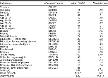
The LMAS data make it possible to consider dummy vari-ables indicating whether the individual was born outside Canada (immigrantD1); whether he or she is disabled and limited at work (disabledD1); his or her age (25–34 is the omitted category); region of residence [three dummy variables for the Atlantic region, Quebec, and Prairies/British Columbia (Ontario is the omitted category)]; and three educational attain-ment dummy variables indicating whether the individual has less education than a high-school diploma (individuals with a high school diploma is the omitted category), has a postsec-ondary diploma, or has a university degree. These variables are included in both estimation stages. In addition, the rst-stage equations include dummy variables indicating whether the in-dividual is married, is the family head, and has his or her own children under age 18. In the wage equation,y2 is the loga-rithm of the hourly wage rate andx2includes, in addition to the aforementioned common variables, the individual’s job tenure, whether he or she is covered by collective bargaining, whether the job has a pension plan, and three dummy variables refer-ring to the employing rm’s size. We have investigated whether

(6)

Table 1. Names and Means of Variables

Full names Shortened names Mean (male) Mean (female)

Constant CONST

Immigrant DBIRTH :11 :10 Disabled DDISAB :04 :04 Age·19 DAGE1 :02 :01 Age 20–24 DAGE2 :10 :10 Age 35–54 DAGE45 :46 :46 Age 55–64 DAGE6 :10 :07 Age 65–69 DAGE7 :01 :01 Atlantic region DREG1 :25 :23 Quebec DREG2 :17 :15 Prairies DREG4 :15 :16 British Columbia DREG5 :24 :25 Education:<High school DEDUC12 :32 :22 Education: Postsecondary diploma DEDUC46 :32 :37 Education: University degree DEDUC5 :24 :25 Married DMARR :75 :74 Family head DHEAD :83 :25 Children OWNKD :15 :13 Tenure (years) TENURE 7:60 5:40 Collective bargaining job DCOLLB :48 :41 Job with pension plan DPPLAN :58 :44 Firm size: 20–99 employees DFMSZ2 :16 :15 Firm size: 100–499 employees DFMSZ3 :13 :14 Firm size: 500Cemployees DFMSZ4 :35 :31 ln (Wage) 2:61 2:34 Hours (annual) 1,937 1,509 Observations 16,891 14,814

xed cost considerations might mean that some variables may enter the participation decision but not the hours equation and found that this was not the case for our data. Therefore, we use the same variables in both the type 2 and the type 3 tobit mod-els. Table 1 lists the names as well as the means for all variables used in the main equations of interest.

A number of regressors in the wage and hours equations may be considered endogenous.Indeed, all but place of birth and age may ultimately be thought of as the outcome of some underly-ing process. Among these variables, education and tenure have attracted the most attention in the literature. Ashenfelter and Rouse (1998) provided a summary of attempts to measure the effects of ability bias (positive) and survey measurement error (negative) on the coefcients, in an OLS context, of education variables. The net effect of these competing forces is close to zero, and its components can be disentangled using such data as education and earnings for monozygotic twins or instruments such as the individual’s quarter of birth. The extent to which OLS equations containing experience (or age) and tenure may underestimate the return to seniority has been examined in the seminal work by Topel (1991), who also proposed a method, based on panel data, for obtaining a lower bound on the return to tenure. (See also Wooldridge 2002, chap. 17, for a detailed dis-cussion on how both the Heckman and Vella–Wooldridge pro-cedures can be combined with IV to allow endogenousexplana-tory variables and sample selection.) The informational require-ments of any attempt to account for the ultimate endogeneity of such explanatory variables far exceed what we have at our dis-posal in the 1989 LMAS, and in any case the focus here is on the application of alternative sample selection techniquesto a prob-lem with a long history in labor economics. We prefer (as many others do) to include such variables as education and tenure in the wage equation and education in the hours equation, because these are important conditioning variables without which t is severely compromised.

4. ESTIMATION RESULTS

4.1 General Issues

We now use the estimators and hypothesis tests outlined ear-lier to obtain selection-adjusted wage equations for men and women. We test for the presence of selection bias and, given that the results suggest that this is an issue that should be taken into account, we consider whether the correcting term in the second stage should be parametric or semiparametric. We also consider the classic Oaxaca (1973) decomposition of wage dif-ferentials for men and women. We restrict our attention to the original Oaxaca (1973) method instead of more recent variants such those of as Cotton (1988) and Oaxaca and Ransom (1994), because our main purpose is to illustrate the new approaches using the most widely used procedure. We estimate the hours equations using probit (normal errors and 0–1 information on hours), Ichimura’s (1993) SNLS method (0–1 information with-out normality), tobit (normal errors and max_f0;y1g informa-tion on hours), Powell’s (1984) CLAD method (normality not assumed), and the n-sample OLS. We estimate the n1 sam-ple wage equations using OLS (ignores selection bias), Heck-man’s (1976, 1979) two-step method, the Vella–Wooldridge (VW) parametric two-step method (u_O1; augmented OLS plus normality) as well as the semiparametric estimators proposed by Chen (1997), HKU (1997), Lee (1994), Li and Wooldridge (2002), Ichimura (1993, denoted by SNLS), and Ichimura and Lee (1991, denoted by IL), as discussed in Section 2. In ad-dition, we also estimate the labor effort and wage equations jointly using the maximum likelihood method (based on joint normality).

Chen (1997) carried out an extensive Monte Carlo study comparing the nite-sample performance of the semiparamet-ric estimators proposed by Chen (1997), HKU (1997), and

(7)

Lee (1994). Chen found that his estimator,¯O2;Chen, performed

competitively relative to the estimators of HKU (1997) and Lee (1994). More recently, Sheu (2000) examined the nite-sample performance of Li and Wooldridge’s (2002) estimator and found that it performs well relative to those of Chen (1997), HKU (1997), and Lee (1994). Thus the existing simulation re-sults suggest that these semiparametric estimators all perform quite well and are robust to different error distributions.

Lee’s method requires a two-dimensional nonparametric kernel estimation and two-dimensional integration. Following Lee (1994, p. 323), we chose a product kernel K.t1;t2/D K₁.t1/K1.t2/withK1.t/D15₁₆.1¡t2/2ifjtj<1 andK1.t/D0 if jt_{j ¸}1. In the product of two univariate kernel functions, the double integrals become the product of two univariate inte-grals, and in theK1.¢/kernel function, the univariate integral has a simple closed-form expression which is a polynomial function. The smoothing parameters used were based on the simple rule of thumbhzDczsdn¡1=6, wherezsd is the standard

deviation offzigniD11 (ziDx1i¯O1 orziD Ou1iDy1i¡x1i¯O1). The Li and Wooldridge (2002) method involves one-dimensional nonparametric kernel estimation; we used the standard normal kernel and chose the smoothing parameters ashzDczsdn¡1=5,

withziD Ou1i. We experimented with cD:8;1:0, and 1:2, but

the results were virtually identical. In the interest of brevity, we report results only for the case ofc_D1.

4.2 The Participation and Hours Equations

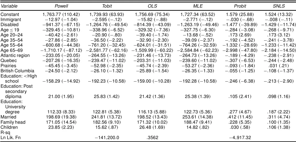
The estimation results for participation and labor supply for men and women are given in Tables 2 and 5. These tables show a striking consistency in the general pattern of results obtained when like is compared with like. Note that the type 2 tobit equa-tion refers to the decision to participate in the labor force or not rather than to the hours supplied, and so the estimated coef-cients will carry a very different meaning than is the case for other estimation procedures.

There are signicant age, region, and education effects. For men, participation is highest for individuals in the age 20–24 class, but working hours is highest for the omitted class of age 25–34. Men in Ontario with university degrees have the highest labor market involvement. For women, participation and hours are both highest for the age 20–24 group, in Ontario and for those with university degrees. Individuals born outside Canada supply less effort, and the disabled supply substantially less ef-fort than the respective control groups. Male married heads who have children work considerably more hours than male single individuals who are not heads and have no children. As is ex-pected, married women with children are able to devote less time to market work.

4.3 The Wage Equations

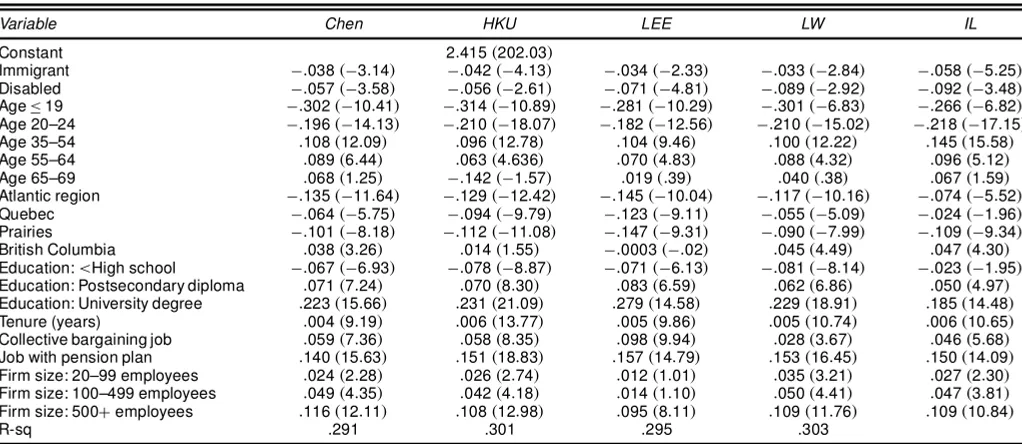
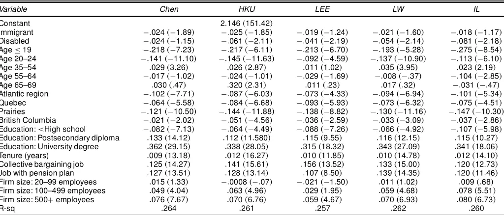
The labor market activity equations in Tables 2 and 5 are of interest in themselves and are also preliminary to the estima-tion of selecestima-tion-adjusted wage equaestima-tions. These equaestima-tions are given in Tables 3 and 4 for males and in Tables 6 and 7 for fe-males. In the case of the semiparametric estimators proposed by Chen (1997), Ichimura (1993), Ichimura and Lee (1991), Lee (1994), and Li and Wooldridge (2002), the intercept term cannot be separately identied. The equations in these tables show substantial consistency in the pattern of regressor signi-cance and size of coefcients. Conicts among the various es-timators concerning the signicance of variables are minimal and are conned to marginally useful variables (e.g., age 65– 69) for both males and females. The age prole of wages for both genders tends to have the familiar concave shape; there are well-established regional effects that differ by gender; the highest-paid males and females reside in British Columbia and Ontario; and more education has the usual positive effect on wages. The tenure variable has a positive and signicant effect that is stronger for females. This is also the case for collective

Table 2. Labor Supply by Males (nD20;316)

Variable Powell Tobit OLS MLE Probit SNLS

Constant 1;763:77.110:42/ 1;739:93.63:93/ 1;756:69.75:34/ 1;727:34.63:52/ 1:579.25:88/ 1:524.13:32/

Immigrant ¡12:97.¡1:04/ ¡2:595.¡:12/ ¡15:82.¡:88/ ¡2:771.¡:12/ ¡:030.¡:68/ ¡:008.¡:11/

Disabled ¡941:37.¡67:15/ ¡1;264:76.¡49:54/ ¡814:39.¡43:09/ ¡1;263:19.¡49:46/ ¡1:477.¡39:89/ ¡1:429.¡11:74/

Age·19 ¡329:45.¡10:81/ ¡338:96.¡6:52/ ¡329:32.¡7:36/ ¡327:75.¡6:30/ ¡:284.¡3:08/ ¡:268.¡9:71/

Age 20–24 ¡40:42.¡2:61/ ¡20:90.¡:80/ ¡39:40.¡1:74/ ¡13:68.¡:52/ :173.2:69/ :173.3:12/

Age 35–54 ¡27:86.¡2:85/ ¡36:50.¡2:22/ ¡32:90.¡2:30/ ¡39:09.¡2:37/ ¡:192.¡4:52/ ¡:241.¡3:78/

Age 55–64 ¡600:68.¡44:36/ ¡761:20.¡32:45/ ¡624:01.¡31:51/ ¡764:26.¡32:59/ ¡1:332.¡28:69/ ¡1:233.¡11:42/

Age 65–69 ¡1;710:17._¡87:12/ _¡2;581:77._¡62:16/ _¡1;509:99._¡60:22/ _¡2;584:84._¡62:23/ _¡2:998._¡47:80/ _¡2:184._¡14:50/

Atlantic region ¡233:05.¡20:05/ ¡264:55.¡13:26/ ¡231:46.¡13:73/ ¡264:73.¡13:26/ ¡:189.¡4:29/ ¡:238.¡2:91/

Quebec ¡207:26.¡16:35/ ¡239:47.¡11:02/ ¡203:31.¡11:03/ ¡239:60.¡11:02/ ¡:307.¡6:53/ ¡:244.¡2:48/

Prairies ¡45:45.¡3:45/ ¡52:98.¡2:35/ ¡45:74.¡2:39/ ¡53:27.¡2:36/ ¡:093.¡1:84/ :031.:21/

British Columbia ¡24:50.¡2:12/ ¡26:10.¡1:32/ ¡25:89.¡1:54/ ¡26:35.¡1:33/ ¡:055.¡1:25/ ¡:108.¡1:37/

Education:<High

school ¡158:29.¡14:92/ ¡192:23.¡10:58/ ¡159:00.¡10:28/ ¡192:28.¡10:58/ ¡:246.¡6:38/ ¡:213.¡2:90/

Education: Post secondary

diploma 21:00.1:95/ 25:83.1:42/ 21:42.1:36/ 25:38.1:39/ :105.2:41/ :098.1:16/

Education: University

degree 112:33.8:33/ 122:81.5:38/ 116:13.5:88/ 122:73.5:36/ :277.4:67/ :187.2:22/

Married 198:69.19:38/ 241:81.13:72/ 198:52.13:43/ 253:61.14:38/ :412.11:45/ :311.4:74/

Family head 171:05.14:54/ 182:56.9:10/ 171:32.10:02/ 188:47.9:41/ :228.5:35/ :100.1:35/

Children 23:85.2:23/ 15:62.:87/ 26:48.1:69/ 14:82.:82/ :030.:58/ :106.1:38/

R-sq

Ln Lik. Fn ¡141;200:0 :3562 ¡4;917:32

NOTE: The values in parentheses are ratios of coefcients to standard errors (tratios).

(8)

Table 3. Wage Equations for Males (parametric, n₁D16;891)

Variable VW Heckman OLS MLE

Constant 2:405.204:40/ 2:425.208:92/ 2:408.210:36/ 2:404.209:98/

Immigrant ¡:041.¡4:28/ ¡:042.¡4:15/ ¡:042.¡4:15/ ¡:041.¡4:12/

Disabled ¡:057._¡3:88/ :146.4:68/ _¡:079._¡5:18/ _¡:044._¡2:74/

Age·19 ¡:303.¡10:99/ ¡:248.¡9:94/ ¡:310.¡12:92/ ¡:301.¡12:56/

Age 20–24 ¡:206._¡17:44/ _¡:203._¡18:15/ _¡:208._¡18:53/ _¡:206._¡18:32/

Age 35–54 :094.13:17/ :102.13:75/ :096.12:99/ :094.12:61/

Age 55–64 :073.5:91/ :209.9:72/ :061.5:08/ :079.6:43/

Age 65–69 :047.:98/ :553.7:51/ :011.:32/ :081.2:34/

Atlantic region ¡:128.¡13:00/ ¡:117.¡12:24/ ¡:129.¡13:61/ ¡:126.¡13:29/

Quebec ¡:087.¡9:58/ ¡:068.¡6:47/ ¡:090.¡8:76/ ¡:086.¡8:38/

Prairies ¡:112.¡11:70/ ¡:108.¡10:24/ ¡:113.¡10:71/ ¡:112.¡10:60/

British Columbia :020.2:19/ :021.2:26/ :019.2:04/ :020.2:18/

Education:<High school ¡:073.¡8:61/ ¡:054.¡6:00/ ¡:076.¡8:83/ ¡:072.¡8:34/

Education: Postsecondary diploma :072.8:80/ :066.7:89/ :073.8:74/ :072.8:59/

Education: University degree :230.20:91/ :218.20:31/ :233.21:99/ :230.21:68/

Tenure (years) :006.14:58/ :005.13:37/ :006.13:82/ :006.14:58/

Collective bargaining job :058.8:44/ :060.8:97/ :061.8:96/ :058.8:57/

Job with pension plan :157.19:95/ :150.19:83/ :152.20:05/ :157.20:63/

Firm size: 20–99 employees :028.3:24/ :027.2:96/ :027.2:98/ :029.3:17/

Firm size: 500Cemployees :109.13:29/ :109.13:60/ :109.13:53/ :109.13:55/

O

¸ _¡:363 (¡8:29)

O

u_1i ¡:00003._¡6:21/

R-sq .301 .302 .299

NOTE: The values in parentheses are the ratios of coefcients to standard errors (tratios).

bargaining coverage. Jobs that offer a pension plan and are with larger rms are more likely to offer higher wages, effects that are also well established in the literature.

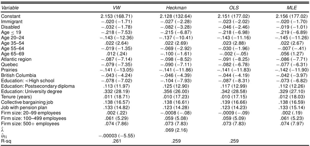
The sample correction variables are signicant for both gen-ders in both the Heckman and Wooldridge approach. The neg-ative selection indicated is a common feature of selection-corrected wage equations (see Baker et al. 1995, p. 490). In-dications that selection effects may be relevant suggest that we consider this issue with care, examining both parametric and semiparametric approaches. This is important because the qual-itative similarity of the results just noted should not be inter-preted as meaning that we should be indifferent as to the esti-mator used. To begin with, this may be a feature of this partic-ular application. In addition, the quantitative evaluation of the

inuence of variables cannot be based simply on the reported coefcient estimates, because many variables also enter the se-lection terms in the wage equations and because their effects on hours necessitate evaluating the effect of variables on probabil-ities of interest. In light of the amount of the calculations that a researcher might wish to undertake, it is particularly important to consider procedures that select the appropriate model, a task to which we now turn.

4.4 Selecting the Correction Procedure

We begin from the general issue of whether sample selection bias is present at all. As already noted, the hypothesis tests in Tables 3 and 6 can be misleading when normality does not hold.

Table 4. Wage Equations for Males (semiparametric, n₁D16;891)

Variable Chen HKU LEE LW IL

Constant 2:415.202:03/

Immigrant ¡:038.¡3:14/ ¡:042.¡4:13/ ¡:034.¡2:33/ ¡:033.¡2:84/ ¡:058.¡5:25/

Disabled ¡:057.¡3:58/ ¡:056.¡2:61/ ¡:071.¡4:81/ ¡:089.¡2:92/ ¡:092.¡3:48/

Age·19 ¡:302.¡10:41/ ¡:314.¡10:89/ ¡:281.¡10:29/ ¡:301.¡6:83/ ¡:266.¡6:82/

Age 20–24 ¡:196._¡14:13/ _¡:210._¡18:07/ _¡:182._¡12:56/ _¡:210._¡15:02/ _¡:218._¡17:15/

Age 35–54 :108.12:09/ :096.12:78/ :104.9:46/ :100.12:22/ :145.15:58/

Age 55–64 :089.6:44/ :063.4:636/ :070.4:83/ :088.4:32/ :096.5:12/

Age 65–69 :068.1:25/ ¡:142.¡1:57/ :019.:39/ :040.:38/ :067.1:59/

Atlantic region ¡:135.¡11:64/ ¡:129.¡12:42/ ¡:145.¡10:04/ ¡:117.¡10:16/ ¡:074.¡5:52/

Quebec ¡:064.¡5:75/ ¡:094.¡9:79/ ¡:123.¡9:11/ ¡:055.¡5:09/ ¡:024.¡1:96/

Prairies ¡:101.¡8:18/ ¡:112.¡11:08/ ¡:147.¡9:31/ ¡:090.¡7:99/ ¡:109.¡9:34/

British Columbia :038.3:26/ :014.1:55/ _¡:0003._¡:02/ :045.4:49/ :047.4:30/

Education:<High school ¡:067.¡6:93/ ¡:078.¡8:87/ ¡:071.¡6:13/ ¡:081.¡8:14/ ¡:023.¡1:95/

Education: Postsecondary diploma :071.7:24/ :070.8:30/ :083.6:59/ :062.6:86/ :050.4:97/

Education: University degree :223.15:66/ :231.21:09/ :279.14:58/ :229.18:91/ :185.14:48/

Tenure (years) :004.9:19/ :006.13:77/ :005.9:86/ :005.10:74/ :006.10:65/

Collective bargaining job :059.7:36/ :058.8:35/ :098.9:94/ :028.3:67/ :046.5:68/

Job with pension plan :140.15:63/ :151.18:83/ :157.14:79/ :153.16:45/ :150.14:09/

Firm size: 20–99 employees :024.2:28/ :026.2:74/ :012.1:01/ :035.3:21/ :027.2:30/

Firm size: 500Cemployees :116.12:11/ :108.12:98/ :095.8:11/ :109.11:76/ :109.10:84/

R-sq .291 .301 .295 .303

(9)

Table 5. Labor Supply by Females (nD23;724)

Variable Powell Tobit OLS MLE Probit SNLS

Constant 1;461:56.35:09/ 1;406:84.40:34/ 1;424:97.61:18/ 1;402:34.40:25/ 1:107.24:48/ 1:947.14:10/

Immigrant ¡39:12.¡1:28/ ¡57:42.¡2:22/ ¡33:75.¡2:05/ ¡57:55.¡2:22/ ¡:103.¡3:35/ ¡:183.¡8:30/

Disabled ¡618:31.¡16:13/ ¡1;054:67.¡31:83/ ¡460:41.¡26:23/ ¡1;054:16.¡31:81/ ¡:968.¡28:18/ ¡1:638.¡14:26/

Age·19 ¡251:15.¡2:96/ ¡273:22.¡3:80/ ¡250:54.¡5:19/ ¡270:38.¡3:76/ ¡:080.¡:94/ ¡:094.¡4:77/

Age 20–24 83:72.2:27/ 106:80.3:50/ 88:27.4:20/ 107:76.3:53/ :168.4:10/ :598.12:54/

Age 35–54 _¡77:98._¡3:33/ _¡109:96._¡5:64/ _¡87:89._¡6:58/ _¡108:75._¡5:58/ _¡:180._¡7:26/ _¡:022._¡1:17/

Age 55–64 ¡659:29.¡20:56/ ¡1;111:49.¡38:91/ ¡642:35.¡36:24/ ¡1;110:02.¡38:86/ ¡1:145.¡36:23/ ¡2:075.¡13:97/

Age 65–69 _¡1;216:74._¡21:55/ _¡2;612:50._¡47:41/ _¡1;008:99._¡46:66/ _¡2;610:69._¡47:38/ _¡2:355._¡42:95/ _¡3:234._¡13:46/

Atlantic region ¡226:20._¡7:90/ _¡299:52._¡12:33/ _¡207:02._¡13:15/ _¡299:44._¡12:32/ _¡:235._¡7:96/ _¡:321._¡9:17/

Quebec _¡172:42._¡5:50/ _¡255:00._¡12:33/ _¡160:51._¡9:28/ _¡254:99._¡9:58/ _¡:265._¡8:21/ _¡:300._¡9:51/

Prairies ¡36:79._¡1:16/ _¡28:51._¡1:07/ _¡30:79._¡1:76/ _¡28:56._¡1:07/ :007.:22/ _¡:046._¡2:47/

British Columbia ¡90:81.¡3:23/ ¡114:51.¡4:81/ ¡84:10.¡5:40/ ¡114:57.¡4:81/ ¡:083.¡2:82/ :022.1:57/

Education:<High

school ¡302:57.¡11:85/ ¡488:88.¡22:25/ ¡272:38.¡19:36/ ¡488:84.¡22:25/ ¡:460.¡18:48/ ¡:993.¡13:98/

Education: Post-secondary

diploma 139:44.5:71/ 196:22.9:55/ 139:60.10:09/ 196:25.9:54/ :251.9:77/ :091.4:41/

Education: University

degree 340:53.10:31/ 451:17.16:40/ 346:76.18:42/ 450:96.16:39/ :566.14:77/ :878.13:09/

Married _¡136:67._¡4:45/ _¡156:77._¡6:09/ _¡116:26._¡6:85/ _¡153:54._¡5:98/ _¡:104._¡3:12/ _¡:251._¡10:44/

Family head 154:49.5:18/ 205:26.8:22/ 134:40.8:13/ 207:54.8:33/ :182.5:63/ :369.11:10/

Children ¡432:94.¡16:49/ ¡579:01.¡26:23/ ¡422:83.¡29:12/ ¡574:20.¡26:06/ ¡:516.¡20:40/ ¡:668.¡12:99/

R-sq .281

Ln Lik. Fn ¡130;618 ¡10;068

We test the null hypothesis of no selection bias,E.u2ju1/D0, against the alternative ofE.u2ju1/´g.u1/6D0. The computed values ofI_naare 12:48 for males and 6:54 for females; because these values exceed the one-tailed critical value of 1:645 at the 5% level, we reject the null of no selection bias for both males and females. We then turn to the particular issue of whether the parametric or semiparametric model is appropriate. We test the null hypothesisE.y2jx2;u1/Dx2¯2Cu1° against the alterna-tive hypothesisE.y2jx2;u1/Dx2¯2Cg.u1/withg.u1/6Du1°. The calculated values of Ib_n are 6:16 for males and 1:31 for

females. Thus we reject Wooldridge’s (1994) linear correction term as the correct specication for males at the 5% level. For the female wage equation, the test fails to reject the parametric null model at the 5% level, but it does reject the null at the 10% level (note that both theI_naand theI_nbare one-sided tests). Thus the results support a semiparametric specication of the wage equation. It is difcult to rank the ve semiparametric methods used based on an empirical application, especially when all of them give similar estimation result. The simulation results of Sheu (2000) showed that Li and Wooldridge’s (2002) estimator

Table 6. Wage Equations for Females (parametric, n₁D14;814)

Variable VW Heckman OLS MLE

Constant 2:153.168:71/ 2:128.132:64/ 2:151.177:02/ 2:156.177:02/

Immigrant ¡:020.¡1:71/ ¡:027.¡2:28/ ¡:023.¡2:02/ ¡:020.¡1:70/

Disabled ¡:032._¡1:78/ _¡:082._¡3:28/ _¡:046._¡2:46/ _¡:019._¡1:01/

Age·19 ¡:218.¡7:53/ ¡:215.¡6:87/ ¡:218.¡6:98/ ¡:219.¡6:89/

Age 20–24 ¡:143.¡12:36/ ¡:137.¡10:41/ ¡:143.¡11:16/ ¡:145.¡11:26/

Age 35–54 :022.2:64/ :022.2:69/ :023.2:88/ :022.2:67/

Age 55–64 ¡:019.¡1:35/ ¡:069.¡2:92/ ¡:030.¡1:96/ ¡:007.¡:41/

Age 65–69 :012.:24/ _¡:100._¡1:61/ _¡:002._¡:05/ :056.1:27/

Atlantic region ¡:087.¡7:14/ ¡:098.¡8:52/ ¡:091.¡8:25/ ¡:086.¡7:71/

Quebec ¡:079._¡7:35/ _¡:090._¡7:11/ _¡:082._¡6:78/ _¡:077._¡6:31/

Prairies ¡:141.¡13:05/ ¡:141.¡11:86/ ¡:141.¡11:83/ ¡:142.¡11:90/

British Columbia ¡:043._¡4:24/ _¡:046._¡4:39/ _¡:044._¡4:19/ _¡:042._¡3:97/

Education:<High school ¡:078.¡7:02/ ¡:104.¡7:93/ ¡:087.¡8:31/ ¡:073.¡6:82/

Education: Postsecondary diploma :113.11:97/ :125.12:90/ :117.12:99/ :112.12:26/

Education: University degree :332.28:19/ :356.26:00/ :342.28:58/ :329.27:10/

Tenure (years) :011.18:71/ :010.17:23/ :010.17:15/ :012.18:03/

Collective bargaining job :138.16:57/ :138.16:61/ :139.16:66/ :138.16:59/

Job with pension plan :133.14:82/ :123.14:28/ :123.14:23/ :133.15:14/

Firm size: 20–99 employees :002.:22/ _¡:0008._¡:08/ _¡:0009._¡:09/ :002.:19/

Firm size: 500Cemployees :074.7:86/ :073.7:83/ :073.7:83/ :074.7:97/

O

¸ .069 (2.16)

O

u_1i ¡:00003.¡5:55/

R-sq .261 .259 .259

(10)

Table 7. Wage Equations for Females (semiparametric, n₁D14;814)

Variable Chen HKU LEE LW IL

Constant 2:146.151:42/

Immigrant ¡:024.¡1:89/ ¡:025.¡1:85/ ¡:019.¡1:24/ ¡:021.¡1:60/ ¡:018.¡1:17/

Disabled ¡:024._¡1:15/ _¡:061._¡2:11/ _¡:041._¡2:19/ _¡:054._¡2:14/ _¡:081._¡2:18/

Age·19 ¡:218.¡7:23/ ¡:217.¡6:11/ ¡:213.¡6:70/ ¡:193.¡5:28/ ¡:275.¡8:54/

Age 20–24 ¡:141._¡11:10/ _¡:145._¡11:63/ _¡:092._¡4:59/ _¡:137._¡10:90/ _¡:113._¡6:10/

Age 35–54 :029.3:26/ :026.2:87/ :011.1:02/ :035.3:95/ :023.2:19/

Age 55–64 ¡:017.¡1:02/ ¡:024.¡1:01/ ¡:029.¡1:69/ ¡:008.¡:37/ ¡:104.¡2:85/

Age 65–69 :030.:47/ :320.2:31/ :011.:23/ :017.:32/ ¡:031.¡:47/

Atlantic region ¡:102.¡7:71/ ¡:087.¡6:03/ ¡:073.¡4:33/ ¡:094.¡6:94/ ¡:101.¡5:34/

Quebec ¡:064.¡5:58/ ¡:084.¡6:68/ ¡:093.¡5:93/ ¡:073.¡6:32/ ¡:075.¡4:51/

Prairies ¡:121.¡10:50/ ¡:144.¡11:88/ ¡:138.¡8:82/ ¡:130.¡11:16/ ¡:147.¡10:30/

British Columbia _¡:021._¡2:02/ _¡:051._¡4:56/ _¡:036._¡2:59/ _¡:033._¡3:09/ _¡:037._¡2:86/

Education:<High school ¡:082.¡7:13/ ¡:064.¡4:49/ ¡:088.¡7:26/ ¡:066.¡4:92/ ¡:107.¡5:98/

Education: Postsecondary diploma :133.14:12/ :112.11:580/ :115.9:55/ :116.12:15/ :115.10:27/

Education: University degree :362.29:15/ :338.28:05/ :315.18:32/ :343.27:09/ :341.18:06/

Tenure (years) :009.13:18/ :012.16:27/ :010.11:85/ :010.14:78/ :012.14:10/

Collective bargaining job :125.14:27/ :141.15:61/ :156.13:52/ :133.15:00/ :120.12:73/

Job with pension plan :127.13:51/ :128.13:14/ :107.8:50/ :139.14:35/ :120.11:46/

Firm size: 20–99 employees :015.1:33/ _¡:0008._¡:07/ _¡:021._¡1:50/ :011.1:02/ :009.:68/

Firm size: 500Cemployees :076.7:67/ :070.6:76/ :059.4:67/ :070.6:93/ :080.6:73/

R-sq :264 :261 :257 :262 :260

compare well with those of Chen (1997), HKU (1997), and Lee (1994). Given this and the fact that all the semiparametric meth-ods lead to similar results, we will only consider results based on the work of Li and Wooldridge (2002) in the next section when discussing wage decompositions.

4.5 Wage Decompositions

One standard application of results such as those in the pre-ceding section is the decomposition of the observed average log-wage differential between males and females into the por-tion attributable to differences in the average values of explana-tory variables and the portion attributable to differences in co-efcients. The latter might be due to discrimination. We present these classic Oaxaca (1973) decompositions using estimates from the various procedures mentioned earlier.

The actual difference in the means of the log-wages for males and females.y_N₂m¡ Ny2f/is:2617 and, in the OLS case

where no selection correction is made, the standard decompo-sition into the term .x_N2m¡ Nx2f/¯2m, which describes the

por-tion attributable to the difference in characteristics plus the term (¯2m¡¯2f/Nx2f which describes the portion possibly attributable

to discrimination results in the amounts:0269 and:2348. That is, only 10:27% of the differential in the mean log-wages can be explained by superior productivity characteristics for males. In the Heckman (1979) approach this percentage is 12:44%, in the Wooldridge (1994) approach it is 10:78%, and in the semi-parametric approach (Li–Wooldridge) it is 9:10%. Nonetheless, the hypothesis tests in the preceding section suggest that the appropriate comparison is between the semiparametric sample-corrected estimates, in which case the explained percentage is 9:10%. Thus all estimators suggest that most of the gender gap cannot be explained by differences in the characteristics that we are able to measure. This consistency suggests some mea-sure of condence in the application of these new procedures to traditional labor market issues.

5. CONCLUSION

Li and Wooldridge (2002) proposed a coherent two-stage strategy for dealing with sample selection problems in a type 3 tobit model that includes the traditional parametric approach of Heckman (1979), Vella (1992), and Wooldridge (1994) as spe-cial cases. This approach follows a general-to-particular strat-egy, rst testing whether sample selection is a problem at all and then testing which particular sample selection procedure (semiparametric or parametric) is appropriate. In contrast to the standardt test of the coefcient on the inverse Mills ratio in the Heckman (1976, 1979) approach, which is problematic when normality does not hold, the tests used here are consis-tent and robust to different distributional assumptions. In this article we have used the estimation method proposed by Li and Wooldridge (2002) as well as the recently proposed semipara-metric methods of Chen (1997), Honore, Kyriazidou and Udry (1997), Ichimura (1993), Ichimura and Lee (1991), and Lee (1994), to analyze data from the 1989 LMAS for Canada. We applied these semiparametric approaches to high-qualitydata to examine labor force involvement and selection-corrected wage equations. We have found that the new procedures produce very reasonable results and conclude that sample selection must be dealt with and that the semiparametric specications are the preferred approach. Using these procedures, we have also ex-amined the standard Oaxaca (1973) decomposition of the gen-der wage gap, and conclude that only a small portion of this gap can be explained by differences in measured productivity characteristics.

ACKNOWLEDGMENTS

We thank two referees, an associate editor, and Jeff Wool-dridge for insightful comments that greatly improved the ar-ticle. We also thank R. Swidinsky, B. Wandschneider, and D. Wang for their helpful comments and advice. This research

(11)

is partly supported by the SSHRC of Canada, the Private Enter-prise Research Center, and the Bush Program in Economics of Public Policy, Texas A&M University. Christodes thanks the University of Guelph, where he is Adjunct Professor.

[Received February 1999. Revised November 2002.]

REFERENCES

Ashenfelter, O., and Rouse, C. (1998), “Schooling, Intelligence, and Income in America: Cracks in the Bell Curve,” Working Paper 407, Princeton Univer-sity.

Baker, M., Benjamin, D., Desaulniers, A., and Grant, M. (1995), “The Distribu-tion of the Male–Female Earnings Differential, 1970–90,”Canadian Journal of Economics, XXVIII, 479–501.

Chen, S. (1997), “Semiparametric Estimation of Type-3 Tobit Model,”Journal of Econometrics, 80, 1–34.

Cotton, J. (1988), “On the Decomposition of Wage Differentials,”The Review of Economics and Statistics, 70, 236–243.

Gronau, R. (1974), “Wage Comparisons: A Selectivity Bias,”Journal of Politi-cal Economy, 82, 1119–1144.

Heckman, J. (1976), “The Common Structure of Statistical Models of Trunca-tion, Sample Selection and Limited Dependent Variables and a Simple Esti-mator for Such Models,”Annals of Economic and Social Measurement, 5/4, 475–492.

(1979), “Sample Selection Bias as a Specication Error,” Economet-rica, 47, 153–161.

(1990), “Varieties of Selection Bias,”American Economic Review, Pa-pers and Proceedings, 80, 313–318.

Honore, B. E., Kyriazidou, E., and Udry, C. (1997), “Estimation of Type-3 Tobit Models Using Symmetric Trimming and Pairwise Comparisons,”Journal of Econometrics, 76, 107–128.

Honore, B. E., and Powell, J. L. (1994), “Pairwise Difference of Linear, Cen-sored and Truncated Regression Models,”Journal of Econometrics, 64, 241– 278.

Ichimura, H. (1993), “Semiparametric Least Squares (SLS) and Weighted SLS Estimation of Single Index Models,”Journal of Econometrics, 58, 71–120. Ichimura, H., and Lee, L. (1991), “Semiparametric Least Squares Estimation of

Multiple Index Models: Single Equation Estimation,” inNonparametric and Semiparametric Methods in Econometrics and Statistics, eds. W. A. Barnett, J. Powell, and G. Tauchen, Cambridge, U.K.: Cambridge University Press, pp. 3–49.

Lee, L. F. (1994), “Semiparametric Two-Stage Estimation of Sample Selection Models Subject to Tobit-Type Selection Rules,”Journal of Econometrics, 61, 305–344.

Lewis, H. (1974), “Comments on Selectivity Biases in Wage Comparisons,”

Journal of Political Economy, 82, 1145–1157.

Li, Q., and Wang, S. (1998), “A Simple Consistent Bootstrap Test for a Para-metric Regression Function,”Journal of Econometrics, 87, 145–165. Li, Q., and Wooldridge, J. (2002), “Semiparametric Estimation of Partially

Lin-ear Models for Dependent Data With Generated Regressors,”Econometric Theory, 18, 625–645.

Manski, C. F. (1989), “Anatomy of the Selection Problem,”Journal of Human Resources, 24, 343–360.

(1990), “Nonparametric Bounds on Treatment Effects,” American Economic Review, Papers and Proceedings, 80, 319–323.

Newey, W. K., Powell, J. L., and Walker, J. R. (1990), “Semiparametric Esti-mation of Selection Models: Some Empirical Results,”American Economic Review, Papers and Proceedings, 80, 324–328.

Oaxaca, R. L. (1973), “Male-Female Wage Differentials in Urban Labour Mar-kets,”International Economic Review, 14, 693–709.

Oaxaca, R. L., and Ransom, M. R. (1994), “On Discrimination and the Decom-position of Wage Differentials,”Journal of Econometrics, 61, 5–21. Powell, J. L. (1984), “Least Absolute Deviations Estimation for the Censored

Regression Model,”Journal of Econometrics, 25, 303–325.

Powell, J. L., Stock, J. H., and Stoker, T. M. (1989), “Semiparametric Estima-tion of the Index Coefcients,”Econometrica, 57, 1043–1430.

Robinson, P. (1988), “Root-N-Consistent Semiparametric Regression,” Econo-metrica, 56, 931–954.

Sheu, S. (2000), “Monte Carlo Study on Some Recent Type-3 Tobit Semipara-metric Estimators,” manuscript, Texas A&M University.

Statistics Canada (1987), “Labour Market Activity Survey,”Microdata User’s Guide1986–87, Longitudinal File (Ottawa).

Topel, R. (1991), “Specic Capital, Mobility, and Wages: Wages Rise with Job Seniority,”Journal of Political Economy, 99, 145–176.

Vella, F. (1992), “Simple Tests for Sample Selection Bias in Censored and Dis-crete Choice Model,”Journal of Applied Econometrics, 7, 413–421.

(1993), “A Simple Estimator for Simultaneous Models With Censored Endogenous Regressors,”International Economic Review, 34, 441–457.

(1998), “Estimating Models With Sample Selection Bias: A Survey,”

Journal of Human Resources, 33, 127–169.

Wooldridge, J. M. (1994), “Selection Corrections With a Censored Selection Variable,” mimeo, Michigan State University.

(1995), “Selection Corrections for Panel Data Models Under Condi-tional Mean Independent Assumptions,”Journal of Econometrics, 68, 115– 132.

(2002),Econometric Analysis of Cross-Section and Panel Data, Cam-bridge, MA: MIT Press.

Zheng, J. X. (1996), “A Consistent Test of Functional Form via Nonparametric Estimation Technique,”Journal of Econometrics, 75, 263–289.