SEISMIC RISK ASSESSMENT OF LEVEES
*Dario Rosidi
Principal Technologist, CH2M HILL Corporation 155 Grand Avenue, Suite 1000 Oakland, CA 94612, USA
Email: [email protected]
ABSTRACT
A seismic risk assessment procedure for earth embankments and levees is presented. The procedure consists of three major elements: (1) probability of ground motion at the site, (2) probability of levee failure given a level of ground motion has occurred and (3) expected loss resulting from the failure. This paper discusses the first two elements of the risk assessment. The third element, which includes economic losses and human casualty, will not be presented herein. The ground motions for risk assessment are developed using a probabilistic seismic hazard analysis. A two-dimensional finite element analysis is performed to estimate the dynamic responses of levee, and the probability of levee failure is calculated using the levee fragility curve. The overall objective of the assessment is to develop an analytical tool for assessing the failure risk and the effectiveness of various levee strengthening alternatives for risk reduction. An example of the procedure, as it applies to a levee built along the perimeter of an island for flood protection and water storage, is presented. Variations in earthquake ground motion and soil and water conditions at the site are incorporated in the risk assessment. The effects of liquefaction in the foundation soils are also considered.
Keywords: Seismic analyses, risk assessment, logic tree, embankment, levee, dynamic response, slope deformation
INTRODUCTION
This paper discusses a seismic risk assessment procedure for earth embankments and levees. The overall objective of the assessment is to develop an analytical tool for assessing levee vulnerability subject to seismic loads and for evaluating effect-tiveness of various levee strengthening alternatives. A general risk assessment procedure consists of three major elements: (1) probability of ground motions at the levee site, (2) probability of levee failure given a level of ground motion has occurred and (3) the expected loss resulting from the failure. This paper presents the first two elements of the risk assessment.
The probabilistic seismic hazard analysis is com-monly used to estimate the ground motions at a site. To compute the levee dynamic responses and the estimated levee deformations, a two-dimensional finite element analysis is performed. The results of these analyses are then combined with the levee fragility curve to provide estimates of the probability of failure.
Because earthquake ground motions at a site are uncertain and levee, soil and water conditions often vary over the levee site and time, the seismic risk is calculated by considering the variation of these factors.
*Also published in the 11th Int. Conf. on Soil Dynamics & EQ
Engng. and the 3rd Int. Conf. on EQ Geotechnical Engng., January
07-09, 2004, Berkeley, California.
Note: Discussion is expected before November, 1st 2007, and will be published in the “Civil Engineering Dimension” volume 10, number 1, March 2008.
Received 5 March 2007; revised 11 April 2007; accepted 19 April 2007.
To help illustrating and discussing the procedure, consider a hypothetical levee built along the perimeter of an island for flood protection and water storage (reservoir). The interior soil stratigraphy in the island consists of a surficial soft organic fibrous peat layer, underlain by a silty sand aquifer. The sand aquifer, in turn, overlies stiff silty clay deposits, and it has the potential to liquefy when subjected to earthquake shaking. The thickness of the peat and sand layers varies from one part of the island to another. The effectiveness of levee strengthening techniques for reducing the risk is also illustrated.
ANALYSIS APPROACH
Seismic risk of a levee is assessed through the probability that the levee will experience one or more failures during future earthquake. The likelihood of a levee experiencing failure is assumed to be a function of seismic-induced slope deformation, expressed in term of levee fragility. The assessment procedure, therefore, consists of three elements: (A) earthquake ground motions, (B) levee deformations and (C) expected levee damage (probability of levee failure). Discussions on these three elements are presented below.
Earthquake Ground Motion
The earthquake ground motion is developed using a probabilistic seismic hazard analysis (PSHA). This analysis procedure was originally developed by Cornell [1] and Kulkarni et al. [2], and includes many recent features/development. It takes into accounts the uncertainties in the size, location and rate of recurrence of earthquakes and in the variation of ground motion characteristics at the site. The major components or steps in a PSHA are:
1. Characterization of seismogenic earthquake sources: the location, geometry and characteristics of seismic sources or earthquake faults.
2. Specification of source recurrence relationship: relationship that shows the annual recurrences of earthquake of various magnitudes, up to the maximum magnitude.
3. Evaluation of probability of distance to rupture: this probability is assessed by considering the geometry of the fault and relationships between rupture dimension and magnitude.
4. Calculation of exceedance using ground motion attenuation equations: the probability that the ground motion parameter Z, from earthquake of a certain magnitude occurring at a certain distance, will exceed a specified level z at the site.
5. Calculation of probabilistic seismic hazard: the mathematical procedure for combining the components described in steps 1 through 4.
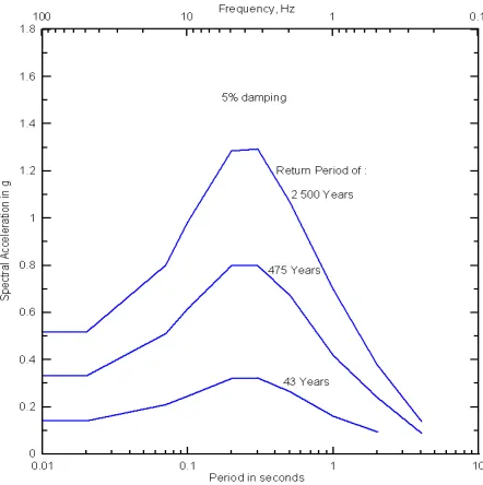
The seismic source model include faults that rupture to the ground surface as well as those that do not (i.e., blind thrust seismic sources). Random or background seismic sources are also included. Proper characterization of uncertainties in source para-meters and ground motion attenuation models is important in a PSHA; they can be incorporated using a logic tree approach, where multiple values of parameters and ground motion models can be considered and weighted. The results of a PSHA are expressed in terms of Uniform Hazard Spectra (UHS) for various exceeding probabilities. Figure 1 shows the calculated UHS for three ground motion return periods: a short period of 43 years, a moderate return of 475 years and a long period of 2,500 years. These UHS represent free-field motions at an outcropping site.
Multiple earthquake acceleration time histories are typically used as inputs to the levee dynamic response analysis. For the purpose of our discussion and illustration, two earthquake time histories are considered. They are selected from the 1992 Landers earthquake (M= 7.3) recorded at Fort Irwin station and the 1987 Whittier Narrows earthquake (M= 6.0) recorded at Altadena, Eaton Canyon station. Table 1 lists these recorded motions along with their closest distances from the rupture planes and the recorded peak accelerations. The 1992 Landers earthquake is selected to represent the larger and more distant
earthquakes, while the 1987 Whittier Narrows earthquake is selected to represent seismic events on the local seismic sources.
Figure 1. Uniform Hazard Spectra for Return Periods of 43, 475, and 2500 Years (Free-Field Stiff Soil)
Table 1. Summary of Earthquake Records Used in the Dynamic Response Analysis
Recording Station
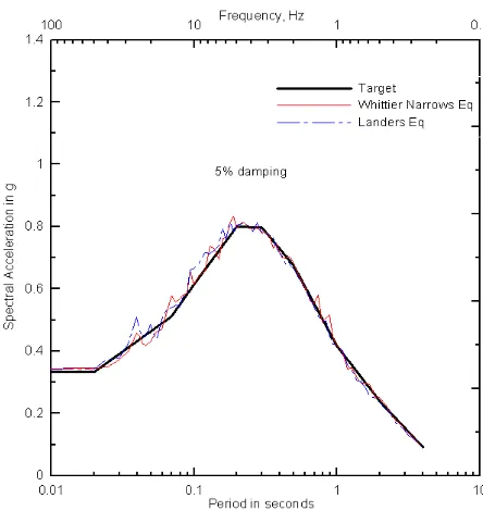
The response spectral ordinates calculated from the recorded acceleration time histories show peaks and valleys that deviate from the smooth UHS. Lilhanand and Tseng [3] proposed a method (later modified by Abrahamson [4]) to develop acceleration time histories with overall characteristics that match the UHS. Using this method, the selected accelera-tion time histories are spectrally matched to the UHS. The 5%-damped response spectra calculated from the modified motions are shown in Figure 2, together with the UHS for the return period of 475 years. This figure indicates that the response spectra calculated from the modified time histories closely match the UHS.
Levee Deformations
The calculation of seismic-induced deformations of a levee consists of the following two steps:
Figure 2. Comparison of Response Spectra for Return Period of 475 Years
Step 1: Site and Levee Dynamic Responses
The earthquake ground motions developed from a PSHA that uses the standard attenuation models are applicable for a free-field stiff soil or rock site. To account for the effects of local soils (fills, organic peat and sand) and levee on the ground motions characteristics, a two-dimensional dynamic response analysis should be carried out. The analysis model should take into accounts the various layers of clayey and sandy soils encountered within and beneath the levee system.
The computer program QUAD4M (Hudson et al. [5]) can be utilized for the analysis. QUAD4M is a two-dimensional, plane-strain, finite element program for dynamic response analysis. It uses the equivalent linear procedure of Seed and Idriss [6] to model the nonlinear behavior of soils. The softening of the soil stiffness is specified using the shear modulus degradation (G/Gmax) and damping vs. shear strain
curves. QUAD4M also incorporates a compliant base (energy-transmitting base), which can be used to model the elastic half-space.
The time histories of seismic-induced inertia forces are calculated from the dynamic response analysis. The average horizontal acceleration (kave) time
history acting on an identified critical sliding mass is then calculated by summing the inertia forces and dividing the sum with the mass of the slide.
Step 2: Seismic-induced Slope Deformations
Seismic-induced permanent slope deformations of a levee can be estimated by the Double Integration Method of Newmark [7]. This method is based on the concept that deformation of a levee will result
from incremental sliding during the short periods when earthquake inertia force in the critical sliding mass exceeds the available resisting force.
The inertia force is calculated using the procedure described above, and the resisting force is represented by the yield acceleration (ky) calculated
for the sliding mass. The yield acceleration of a sliding mass is defined as the horizontal acceleration that will initiate slide movement. This method involves the calculations of the displacement (deformation) increment of a critical sliding mass at each time step using the average horizontal acceleration (kave) and the value of yield acceleration
(ky) calculated for the sliding mass.
The effects of liquefaction on the estimated slope deformations can be incorporated through the reduction in shear resistance along the critical slip surface during earthquake shaking. This translates into lower yield acceleration, ky, which in turn,
induces larger deformations.
Expected Damage
As indicated earlier, the levee probability of failure is assumed to be a function of levee slope deformations (i.e., the levee fragility is expressed as a relationship between probability of levee failure and expected slope deformations). The conditions that define a levee failure include, among others, piping, over-topping, cracking, slumping and excessive settle-ment. Example of a levee fragility curves is presented in Figure 3.
Figure 3. Example of a Levee Fragility Curve
To illustrate the application of the above risk assessment procedure, consider a hypothetical levee system that was built along the perimeter of an island for flood protection and water storage
(reservoir). The existing levee materials generally consist of peat and dredged sand, silt and clay. Beneath the levee is a thick layer of peat with sandy silt inter-layers. This peat is typically about 20 ft
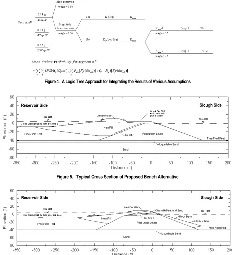
Figure 4. A Logic Tree Approach for Integrating the Results of Various Assumptions
Figure 5. Typical Cross Section of Proposed Bench Alternative
(609.6 cm) to 40 ft (1,219.2 cm) thick in the fields away from the levee, but it has been highly com-pressed under the weight of the levee. Underlying the peat, there is loose to dense sand stratum. In some areas, this sand deposit is susceptible to liquefaction under the expected earthquake shaking.
Two cross sections representing different subsurface conditions along the levee system are developed and used for the analysis: peat extends to elevation –20 ft (-609.6 cm) in one section and extends to elevation –40 ft (-1219.2 cm) in the second section. The weights for these two sections used in the logic tree of risk assessment are assigned based on the percentages of the respective conditions encountered along the levee system.
In addition to the existing levee condition, two levee strengthening alternatives are also considered to evaluate the effectiveness of these strengthening alternatives. The two strengthening alternatives involve:
1. Construction of a new bench (called bench alternative), as shown in Figure 5.
2. Placement of a rock-berm (called rock-berm alternative), as shown in Figure 6.
For the site and levee dynamic response analysis, the shear and compressive wave velocities obtained from a geophysical measurement at the site are used. The relationship that relates maximum shear modulus, over-consolidation ratio (OCR) and effective pressure proposed by Wheling et al. [8] is also utilized to account for the dependency of shear modulus (or shear wave velocity) on effective pressure.
Tabel 2. Dynamic Material Properties
Description
1. Relationships of Kokusho (1980), function of confining pressure 2. Relationships of Wehling et al (2001)
3. Relationships of Vucetic and Dobry (1991) for PI = 50
4. Shear wve velocity ws estimated using the following equations (Wehling et al. 2001)
Where Pa and σ’lc are the atm ospheric and effective vertical pressures, respectively
5. For liquefied sand, no reduction in G is allowed and the damping is fix ed t 8%-10% of critical damping
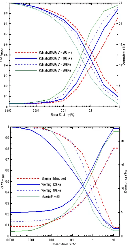
The shear modulus degradation (G/Gmax) and
dam-ping curves of Kokusho [9] and Vucetic and Dobry [10] are applied for the sandy soils (levee fill and alluvium) and clays, respectively. For peat, the relationships of Wheling et al. [8] are utilized. The dynamic soil properties used for the response analyses are summarized in Table 2. Plots of the
selected G/Gmax and damping vs. shear strain
relationships are presented in Figure 7.
Figure 7. Modulus and Damping Curves for Soils Used in Analysis
within these loose sandy deposits during earthquake will increase the levee deformations, and hence the probability of levee failure.
The liquefied shear strength at small strains for the loose sandy deposits is modeled using a shear wave velocity of 300 ft (9144 cm)/sec. No shear modulus degradation is allowed for the liquefied soil condition. The damping values are kept constant at 8% to 10% of the critical damping value. The damage assessment considers the effects of liquefaction, and the weights for the liquefaction scenarios used in the logic tree (Figure 4) are selected based on judgment and evaluation of field blow-counts recorded in the sandy deposits.
Two operating water elevation scenarios are selected to represent the normal fluctuation of surface (reservoir) water and tidal water elevations near the levee. These scenarios are as follows:
1. High Tide and Low Reservoir: a low storage (reservoir) and high slough (tide) water at elevation +3.5 feet. (106.68 cm) This condition was assumed to prevail 2/3 of the time (weight of 0.66).
2. Low Tide and High Reservoir: high storage (reservoir) water at elevation +4.0 feet (121.92 cm) and low slough (tide) water at elevation –1 foot (-30.48 cm). This condition was assumed to prevail 1/3 of the time (weight of 0.34).
Weights assigned to the reservoir and slough water level scenarios are estimated based on the time percentage of each scenario to occur annually.
Figure 8 - Probability of Failure for Existing, Bench, and Rock Berm Alternatives
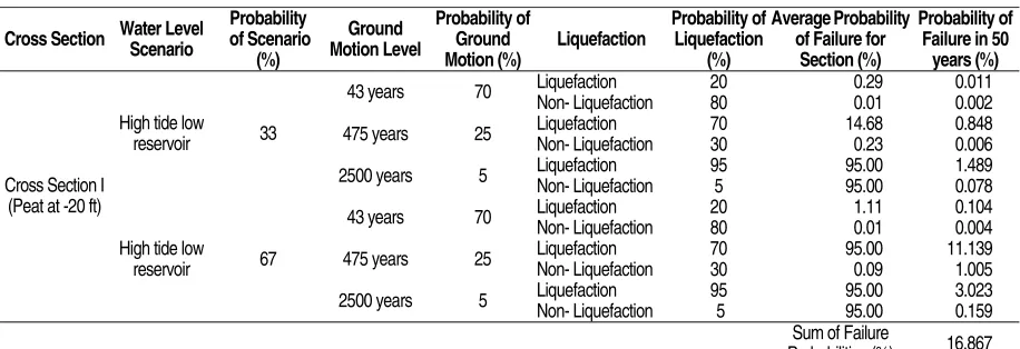
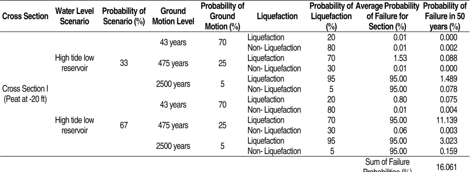
Table 3 shows the contributions of the various scenarios to the expected damages (probabilities of failure) for the existing levee condition with peat extending to elevation -20 ft (60 cm). The total failure probability for this case is estimated to be about 22.24 percent. The corresponding failure proba-bilities for the bench and rock-berm strengthening alternatives are calculated to be about 16.87 percent and 16.06 percent, respectively (Tables 4 and 5).
No comergence
Table 3. Probability of Failure of Existing Cross Section I (Peat At -20 Ft)
Cross Section Water Level Scenario
Probability of Failure for
Section (%)
Probability of Failure in 50
years (%)
Liquefaction 20 2.35 0.329
43 years 70 Non- Liquefaction 80 0.04 0.022
Liquefaction 70 95.00 16.625
475 years 25 Non- Liquefaction 30 6.78 0.509
Liquefaction 95 95.00 4.513
Cross Section I (Peat at -20 ft)
High tide low
reservoir 100
2500 years 5 Non- Liquefaction 5 95.00 0.238
Sum of Failure
Probabilities (%) 22.235
Table 4. Probability of Failure of Cross Section I (Peat At -20 Ft) With Bench Alternative
Cross Section Water Level Scenario
Probability of Failure for
Section (%)
Probability of Failure in 50
years (%)
Liquefaction 20 0.29 0.011
43 years 70 Non- Liquefaction 80 0.01 0.002
Liquefaction 70 14.68 0.848
475 years 25 Non- Liquefaction 30 0.23 0.006
Liquefaction 95 95.00 1.489
High tide low
reservoir 33
2500 years 5 Non- Liquefaction 5 95.00 0.078
Liquefaction 20 1.11 0.104
43 years 70 Non- Liquefaction 80 0.01 0.004
Liquefaction 70 95.00 11.139
475 years 25 Non- Liquefaction 30 0.09 1.005
Liquefaction 95 95.00 3.023
Cross Section I (Peat at -20 ft)
High tide low
reservoir 67
2500 years 5 Non- Liquefaction 5 95.00 0.159
Sum of Failure
Probabilities (%) 16.867
Existing
Bench
Rock Berm
Ground Motion Return Period, years
The calculated failure probabilities for the two strengthening alternatives and the existing levee are compared in Figure 8, as a function of earthquake ground motion return period.
As expected, the strengthening is expected to reduce the risk of levee failure during the design life-time of the levee. The rock-berm alternative produces a lower expected damage (probability of failure) than the bench alternative. This is true because the rock-berm alternative places the embankment over the existing levee, and therefore, makes use of the stronger peat under the levee as opposed to the weaker free-field peat. In addition, it provides a more stable slough side slope.
CONCLUSIONS
The seismic risk assessment procedure described in this paper provides a systematic procedure for
quantifying risk of a levee system, subject to
earthquake loading. The procedure can be used as an efficient/effective tool for decision making. The procedure takes into account the uncertainties associated with earthquake loading and soil and water conditions. It can be used to evaluate various design alternatives, and to help identifying the alternative that produces the lowest risk.
REFERENCES
1 Cornell, C.A., Engineering Seismic Risk Analysis in Bulletin of the Seismological Society of America, 1968, vol. 58, No.5, pp.1583-1606.
2 Kulkarni, R. B., Sadigh, K., and Idriss, I. M., 1979, Probabilistic evaluation of seismic expo-sure, Proceedings, Second U. S. National Confe-rence on Earthquake Engineering, Stanford, California, August 22-24, 1979, pp. 90-99.
3 Lilhanand, K. and Tseng, W.S., Development and Application of Realistic Earthquake Time Histories Compatible with Multiple-Damping Design Spectra. Proceeding of the 9th World
Conference on Earthquake Engineering, Tokyo-Kyoto, Japan, August 1988.
4 Abrahamson, N., Non-Stationary Spectral
Matching Program Personal Communication,
1993.
5 Hudson, M., Idriss, I.M., Beikae, M., User’s Manual for QUAD4M, Center for Geotechnical Modeling, Department of Civil & Environmental Engineering, University of California, Davis, California, May 1994.
6 Seed, H.B. and Idriss, I.M., Soil Moduli In Damping Factors For Dynamic Response Analysis, Report No. EERC 70-10, University of California, Berkeley, December 1970.
7 Newmark N.M., Effects of Earthquakes on Dams and Embankments, Geotechnique, Vol. 15, No. 2, June 1965.
8 Wheling, T.M., Boulanger, R.W., Arulnathan, R., Harder, L.F., and Driller, M.W., Nonlinear Dynamic Properties of a Fibrous Organic Soil,
Journal of Geotechnical and Geoenvironmental Engineering, ASCE, 2001.
9 Kokusho T., Cyclic Triaxial Test of Dynamic Soil Properties for Wide Strain Range, Journal of Soils and Foundations, 1980, Vol. 20, pp. 45-60.
10 Vucetic, M. and Dobry, R., Effect of Soil Plas-ticity on Cyclic Response, Journal of Geotech-nical Engineering, ASCE, 1991, Vol. 117, No.1.
11 NCEER, Proceeding of the NCEER Workshop on Evaluation of Liquefaction Resistance of Soils, edited by Youd, T.L., and Idriss, I.M., 1997, Technical report NCEER-97-0022.
Table 5. Probability of Failure of Cross Section I (Peat At -20 Ft) With Rock Berm Alternative
Cross Section Water Level Scenario Probability of Scenario (%) Motion Level Ground
Probability of of Failure for
Section (%)
Probability of Failure in 50
years (%)
Liquefaction 20 0.01 0.000
43 years 70
Non- Liquefaction 80 0.01 0.002
Liquefaction 70 1.53 0.088
475 years 25 Non- Liquefaction 30 0.01 0.000
Liquefaction 95 95.00 1.489
High tide low
reservoir 33
2500 years 5
Non- Liquefaction 5 95.00 0.078
Liquefaction 20 0.80 0.075
43 years 70
Non- Liquefaction 80 0.01 0.004
Liquefaction 70 95.00 11.139
475 years 25 Non- Liquefaction 30 0.06 0.003
Liquefaction 95 95.00 3.023
Cross Section I (Peat at -20 ft)
High tide low
reservoir 67
2500 years 5 Non- Liquefaction 5 95.00 0.159
Sum of Failure