INTEGRATION OF RS/GIS FOR SURFACE WATER POLLUTION RISK MODELING.
CASE STUDY: AL-ABRASH SYRIAN COASTAL BASIN
A. Yaghi a, H. Salim b a
General Organization of Remote Sensing, Damascus – Syria ( [email protected] ) b
General Organization of Remote Sensing, Damascus – Syria ( [email protected])
KEY WORDS: Point Source Pollution (PSP), non-point Source pollution (NPSP), RS, GIS and pollution risk maps
ABSTRACT:
Recently the topic of the quality of surface water (rivers – lakes) and the sea is an important topics at different levels. It is known that there are two major groups of pollutants: Point Source Pollution (PSP) and non-point Source pollution (NPSP).
Historically most of the surface water pollution protection programs dealing with the first set of pollutants which comes from sewage pipes and factories drainage.
With the growing need for current and future water security must stand on the current reality of the coastal rivers basin in terms of freshness and cleanliness and condition of water pollution.
This research aims to assign the NPS pollutants that reach Al Abrash River and preparation of databases and producing of risk Pollution map for NPS pollutants in order to put the basin management plan to ensure the reduction of pollutants that reach the river.
This research resulted of establishing of Databases of NPSP (Like pesticides and fertilizers) and producing of thematic maps for pollution severity and pollution risk based on the pollution models designed in GIS environment and utilizing from remote sensing data.
Preliminary recommendations for managing these pollutants were put.
1. Introduction
Recently, increasing public awareness about water quality is a major trend. It is well known that Point Source (PS) as well as Nonpoint Source (NPS), or diffuse, sources of pollution are recognized to be the leading causes of water body pollution. PS loading originates from confined areas, such as discharge pipes in factories or sewage plants. NPS loading is carried by storm water runoff and percolating water draining residential, commercial, rural, and agricultural areas where many everyday activities add polluting substances to the land. Historically, most pollution control programs have initially dealt only with PS pollution; however, all over the world and for several decades, a large percentage of water pollution has been recognized as originating from many NPSs (Novotny 1999). Typically, in less developed countries, PSs such as sewage from urban areas and NPSs such as sedimentation from deforestation or agricultural practices are the main components of pollution. In developed countries, runoff from agriculture and urban sources are the leading causes of nonpoint pollution (Luzio, et al., 2004).
The control and management of water quality, particularly for impaired streams where NPSs are the overwhelming sources, would require outrageously expensive monitoring activities. The modeling alternative requires the description and understanding of several hydrologic phenomena with intrinsic spatial and temporal variation. Mathematical, hydrology-based, distributed parameter simulation models and GIS technology provide a potential synergy that appears to be the key feature for an effective under-standing and interpretation of these
complicated hydrologic processes connected with water quality assessment. There are diverse elements promoting the development of such systems for water resources applications (Wilson et al. 2000).
In the case of availability and quality of supporting datasets provide convenient descriptions of important hydrologic variables that are related to chemicals, soils, climate, topography, land cover, and land use.
These elements will ultimately increase the reliability of decision support tools on a watershed scale, the hydrological unit where NPSs and PSs are required to be correctly factored into an effective management system, as all human and natural activities upstream have the potential to affect water quality and quantity downstream.
Agricultural pollution is difficult to monitor since all pollution sources are non-point in nature. The non-point source pollution (NPSP) has long been a major concern all over the world. The USEPA noted in 1990 that routine agricultural activities were responsible for more than 60% of the surface water pollution problems in the US. The importance of agricultural NPSP control has frequently been emphasized in the reports of Environment Canada and Canadian Environmental Assessment Agency even related figures are not available.
The primary requirements for GIS in NPSP modeling can be identified with respect to the features of the modeling work (Hamlett et al. 1992; Engel et al., 1993; Tim and Jolly, 1994; Srinivasan and Engel 1994; Srivastava et al., 2001; Luzio et al. 2004; Yaghi et al. 2012, 2013). As suggested by previous studies on agricultural NPSP with GIS application, a GIS for this area should be capable of performing complex manipulation and analysis of spatial and non-spatial data for the development and preparation of data inputs to models, providing the linkage mechanisms between models having different spatial representation, facilitating the conversion and standardization of data in digital form of different scales and coordinate systems, and enabling post-simulation analysis through graphical display and spatial statistical summaries that facilitate explanation of modeling results.
NPSP modeling is concerned with the movement of pesticides and nutrients, as well as soil erosion. As described by Engel et al. (1993) for agricultural watershed modeling, distributed parameter models incorporate the variability in landscape features that control hydrologic flow and transport process, and thus, are potentially more realistic.
The objectives of this study are to:
1. Designing a GIS Model for monitoring the NPSP from the agricultural sources like fertilizers and pesticides.
2. Establishing the data set in a format suitable to be entered to the GIS model easily.
3. Run the model and get the agricultural pollution risk map for the basin in the year 2011 as the land use map is for this year.
2. Study Area 2-1- Location
Al Abrash river basin is one of the Syrian Coastal Zone Basins. It is approximately 45 kilometers long and 5 to 10 kilometers wide starts from north east in the mountainous area and ends in the South West at the sea line. Al Abrah Basin includes parts of three Governorates (Tartous, Homs and Hama). This area encompasses about 235 square-kilometers.
2-2- Geomorphology
The Basin is geomorphologically divided into three Parts (Figure 1):
• Upper basin: is a mountainous area, with altitude of 1100 -400 m
• Middle Basin: is the hilly area, with altitude of 400 – 100 m
• Lower Basin: plain area, with altitude less than 100 m
Figure 1: Geomorphology of the study area 2-3- Climatology
The climate in the study area is a Mediterranean climate. The participation is between 700 and 1400 mm per year. The average temperature is 13 centigrade degree for the coldest month and 28 centigrade degree for the hottest month. 2-4- Land use
Arable land is about 65% from the total basin land followed by the forest land with 21%, urban 5%, water bodies 5% and others 4%.
The arable land is classified as: olives plantation 57% – citrus 7% – green houses 4% – crops 25% - apple 7%
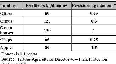
The fertilizers and pesticides are applies in the arable land are illustrated in table (1).
Pesticides kg / donom * Fertilizers kg/donom*
Land use
0.25 60
Olives
0.3 125
Citrus
1 120
Green houses
0.75 65
Crops
1.5 80
Apples
Donom is 0.1 hectar
Source: Tartous Agricultural Directorate – Plant Protection Section (2012)
Table (1): Average Fertilizes (Phosphorous, Nitrogen and Potassium) and Pesticides Loads by Land Use in Al –
Abrash River Basin (kg/Donom)
3. Materials and Methods 3-1 Materials:
Satellite images (rapid eye 2011 – IKONOS 2012) DEM (30 m resolution)
Topo maps 1/25000 Arc/GIS
ERDAS GPS
Maas et al. (1985) show that areas of severe soil loss are often the critical areas for agricultural non-point source pollution. Schauble (1999) mentions that erosion includes not only the transport of sediment particles but also the transport of nutrients and pollutants. Both mechanisms depend on the amount of surface runoff and are therefore linked together. Both processes can only be lessened by reducing the surface runoff in favor of ground water infiltration. Due to this inseparability of both processes, erosion models can be used to find critical areas of non-point source pollution also. For modeling erosion, many models have been developed. De Roo (1993) gives an overview of some important models: universal soil loss equation (USLE; Wischmeier and Smith, 1978), revised USLE (RUSLE; Renard et al 1991), modified USLE (MUSLE87; Hensel and Bork, 1988), areal non-point source watershed environment response system (ANSWERS; Beasley and Huggins, 1982) and agricultural non-point source pollution model (AGNPS; Young et al., 1987). Many of the newer models are derived from the basic USLE of Wischmeier and Smith (1978). This equation is the result of empirical long-term runoff studies on test fields in the USA. It estimates the long-term annual soil loss in [tons/ha]. The formula consists of multiplied factors and is as follows:
A = R*K*L*S*C*P The factors are:
A: result: mean long-term annual soil loss in [tons/ha] R: rain and surface runoff factor
K: soil erodibility factor L: slope length factor S: slope steepness factor C: vegetation cover factor P: erosion protection factor 3-3 Methodology
GIS was used to:
– produce Hydrology maps using ARC/HYDRO.
– produce rainfall map and pollution map using Geo-statistical analyst
– produce SLOPE & ASPECT using SPATIAL ANALYST & 3D
– NPSP modeling
RS (satellite images) was used to: produce Land Cover / Land use maps.
GPS was used to: assign some important locations (environmental points, soil measurements……)
In this research we performed rough analyses to reveal critical erosion and non-point source pollution areas using the advantages of a GIS, and used a modified USLE model (Sivertun et al., 1988). That model combined four factor maps by simple raster value multiplication to produce a risk map. Weights for every factors were established based on the literature review of similar researches and the experiences of the researcher (Yaghi et.al., 2012- 2013). The formula used is as follows:
P = K*S*W*U The maps are:
P: product map, showing the risk of erosion and pollution K: soil factor map
S: slope factor map W: watercourse factor map U: land use factor map
In contrast to the original USLE, the product map of the modified USLE does not give information on the actual sediment or pollution load, but it allows one to find places with a high risk of erosion or influence on surface water quality in the investigation area.
Table 2 shows the values of the factor maps. The model has been chosen for this work because it gives a fast overview of the critical areas, which can later be analyzed more profoundly with a more sophisticated technique. An advantage is the time and cost saving. Updating is also easy: if more accurate maps are available or the land cover changes, it does not influence the other factor maps. The model can be recalculated easily after changing one factor map. Thus, the model can be used for long-term studies within the scope of sustainable development (Schein and Sivertun, 2001 ; Yaghi et al. 2012 -2013). It is illustrated in Figure (2) and table (2).
Figure (2): Flow chart of the pollution risk modeling
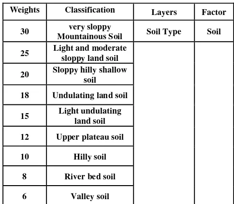
Factor Layers
Classification Weights
Soil Soil Type
very sloppy Mountainous Soil 30
Light and moderate sloppy land soil 25
Sloppy hilly shallow soil 20
Undulating land soil 18
Light undulating land soil 15
Upper plateau soil 12
Hilly soil 10
River bed soil 8
Alluvial soil 4
Plain soil 2
1100 – 1200 mm 10
1200 – 1300 mm 15
1300 – 1400 mm 20
1400 -1500 mm 25
1500 – 1600 mm 30
Distance from Drainage Drainage
0
1- 100 m 10
011 – 511 m 9
511 - 011 m 8
011 – 0011 m 6
0011 – 5111 m 3
More than 5111 m 1
Table 2: Factors and weights entered to the model of surface water pollution risk map
4. Results
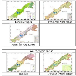
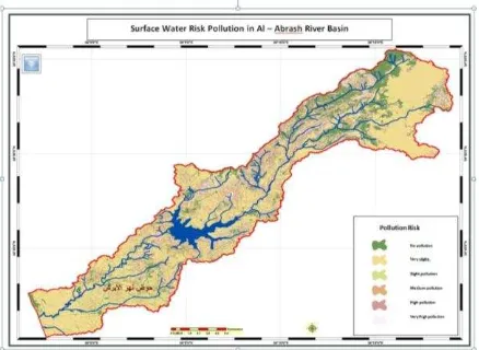
Based on the results of multiplication of factor maps (Figure 3), we classified the results into five surface water pollution risk classes. Table (3) and figure (4) illustrate the result of this research.
Soil Factor
Soil Type Soil Depth
Slope Factor
Slope Gradient Slope Length
Land Cover /land use Factor
Land use Types Fertilizers Application
Pesticides Application
Figure 3: Factors maps of the proposed model
Percentage Area (m)
Weights multiplication Pollution
Risk Level
20.28 47516.5
0 Not
Relevant 1
45.98 107747.4
Less than 5000 Very slight
pollution Risk 2
7.91 18537.8
5000 - 10000 Slight
Pollution Risk 3
14.16 33177.9
10000 - 25000 Medium
Pollution Risk 4
6.58 15418.0
25000 - 50000 High
Pollution Risk 5
5.09 11917.4
More than 50000 Very high
Pollution Risk 6
100 234314.97
Table 3: surface water pollution risk classes, areas and percentages
Water course Factor
Figure 4: surface water pollution risk map:
5. Conclusion
In this paper, we presented and concluded the following: • The powerful of GIS modeling for producing surface
water pollution risk map of nonpoint source pollution on a watershed scale.
• The derived surface water pollution risk map can be updated every time we can get more accurate or updated land use maps.
• Based on the model applied, Al - Abrash Basin was divided into 5 surface water pollution risk classes. Locations, areas and percentage of every class were calculated.
• The method can be applied for all coastal rivers basins.
• GIS can also used to select the best locations for water analysis in order to know the concentration of the pollutants though the time (water monitoring plan).
• The result of such kind of research can be used in the integrated land management and in managing sedimentations, nutrients and pesticides measures in the coastal zone.
References
Beasley, D.B., Huggins, L.F., 1982. ANSWERS. Department of Agricultural Engineering, Purdue University, West Lafayette, USA.
De Roo, A.P.J., 1993. Modelling Surface Runoff and Soil Erosion in Catchments Using Geographical Information Systems. Faculteit Ruimtelijke Wetenschappen, Universiteit Utrecht, Netherlands.
Engel, B. A. et al. (1993): A Spatial Decision Support System for Modeling and Managing Agricultural Non-Point Source Pollution. Environmental Modeling with GIS, Goodchild, M. F. et al. (eds.), New York, Oxford University Press, 231-237. Hamlett, J. M. et al. (1992). Statewide GIS-based ranking of watersheds for agricultural pollution prevention. J. Soil and Water Conservancy, 47(5), 399-404.
Hensel, H., Bork, H.R., 1988. Computer aided construction of soil erosion and deposition maps. Geol. Jahrb. A 104, 357–371.
Luzio M D, Srinivasan R, and Arnold J G., 2004. A GIS-Coupled Hydrological Model System for the Watershed Assessment of Agricultural Nonpoint and Point Sources of Pollution. Transactions in GIS, , 8(1): 113-136
Maas, R.P., Smolen, M.D., Dressing, S.A., 1985. Selecting critical areas for non-point source pollution control. J. Soil Water Conserv. 40 (1), 68–71.
Novotny V 1999. Diffuse pollution from agriculture: A worldwide outlook. Water Science and Technology 39: 1-13 Schauble, 1999. Erosionsprognosen mit GIS und EDV—Ein Vergleich verschiedener Bewertungskonzepte am Beispiel einer Ga¨ulandschaft. Geographisches Institut, Universita¨t Tu¨bingen, Germany.
Schein, T., Sivertun, A., 2001. Method and models for sustainable development monitoring and analyses in GIS. In: Proceedings of the International Workshop on Geo-Spatial Knowledge Processing for Natural Resource Management, University of Insubria, Varese, Italy.
Sivertun, A., et al. 1988. A GIS method to aid in non-point source critical area analysis. Int. J. Geogr. Inf. Syst. 2 (4), 365– 378.
Srinivasan R. and Engel, B. A. (1994). A Spatial Decision Support System for Assessing Agricultural Nonpoint Source Pollution. Water Resources Bulletin, 30, 3, 441-452.
Srivastava P., Day R.L., Robillard P.D., and Hamlett J.M. (2001). AnnGIS: Integration of GIS and a Continuous Simulation Model for Non-Point Source Pollution Assessment. Transactions in GIS 5(3) 221-234.
Tim, U S and Jolly R. (1994). Evaluating Agricultural Nonpoint-Source Pollution Using Integrated Geographic Information System and Hydrologic/Water Quality Model. J. Environ. Quality, 23, Jan.-Feb., 25-35.
Wilson J P, Mitasova H, and Wright D J 2000 Water resource applications of Geographic Information Systems. Journal of the Urban and Regional Information Systems Association 12: 61-79.
Wischmeier, W.H., Smith, D.D., 1978. Predicting Rainfall Erosion Losses. Agricultural Handbook 537. US Department of Agriculture, Washington, DC, USA.
Wu ., Li ., Huang G. 2005. GIS Applications to Agricultural Non-Point-Source Pollution Modeling: A Status Review. Environmental Informatics Archives, Volume 3, 202 – 206 Yaghi., A., |(2012) Integrated Environmental Management of Al Kabeer Al Shamali River Basin. Report. General Organization of Remote Sensing – Damascus - Syria
Yaghi., A., |(2013) Integrated Environmental Management of Al Abrash River Basin. Report. General Organization of Remote Sensing – Damascus - Syria