DETECTION OF PERSONS IN MLS POINT CLOUDS USING IMPLICIT SHAPE
MODELS
B. Borgmanna,b∗, M. Hebela, M. Arensa, U. Stillab
a
Fraunhofer IOSB, Gutleuthausstr. 1, 76275 Ettlingen, Germany (bjoern.borgmann, marcus.hebel, michael.arens)@iosb.fraunhofer.de
bTechnical University of Munich, Dept. of Photogrammetry and Remote Sensing, Arcisstr. 21, 80333 Munich, Germany
KEY WORDS:LiDAR, Mobile, Laser scanning, Person, Detection, Classification
ABSTRACT:
In this paper we present an approach for the detection of persons in point clouds gathered by mobile laser scanning (MLS) systems. The approach consists of a preprocessing and the actual detection. The main task of the preprocessing is to reduce the amount of data which has to be processed by the detection. To fulfill this task, the preprocessing consists of ground removal, segmentation and several filters. The detection is based on an implicit shape models (ISM) approach which is an extension to bag-of-words approaches. For this detection method, it is sufficient to work with a small amount of training data. Although in this paper we focus on the detection of persons, our approach is able to detect multiple classes of objects in point clouds. Using a parameterization of the approach which offers a good compromise between detection and runtime performance, we are able to achieve a precision of 0.68 and a recall of 0.76 while having a average runtime of370 msper single scan rotation of the rotating head of a typical MLS sensor.
1. INTRODUCTION
The detection of pedestrians (or more general persons) in data which are gathered by mobile laser scanning (MLS) systems is a useful functionality for several use cases. It is, for example, help-ful for the save navigation of an autonomous vehicle or the save operation of an autonomous machine in the vicinity of people. It can also be part of a driver assistance system or an assistance system for the operator of a large machine. Such an assistance system could increase the safety of operation if such a machine is used around people. Of course there are also many use cases in the area of human-robot interaction.
Unlike the general detection of obstacles or moving objects, the actual detection of people allows paying particular attention to their safety. An autonomous vehicle can, for example, keep an extra distance to persons or, if a collision could not be avoided, it could be preferable to collide with a wall instead with a person.
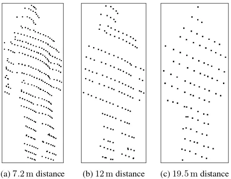
There are several challenges to deal with for the detection of per-sons in use cases like the ones mentioned above. One is that even with modern mobile laser scanning systems the resulting data density of single scans is comparatively low so that often a person is only comprised of 100 - 200 single point measurements. This is demonstrated in Figure 1, which shows a person in differ-ent distances in single scans of a LiDAR sensor which is typically used in MLS systems. Another challenge is that many of the use cases depend on real time processing, meaning that the person detection method should be able to process data in the speed of data acquisition. This limits the computational complexity of the method.
2. RELATED WORK
There are several existing approaches to detect persons or more generally speaking, recognize certain object classes in
LiDAR-∗Corresponding author
(a)7.2 mdistance (b)12 mdistance (c)19.5 mdistance
Figure 1. Person in a single scan of a Velodyne HDL-64E LiDAR in different distances.
Another kind of classifiers are random decision forests. These utilize several decision trees at once and train them with a cer-tain random element. This allows them to deal with the problem of overfitting. Their classification result is generated by merg-ing the results of the different decision trees. They are, for ex-ample, used to detect persons and body parts of the persons in depth images generated by Microsoft’s KINECT sensor by clas-sifying each pixel of the depth image. They are able to do that in the speed of data acquisition but need depth images with a suf-ficiently high resolution and a large amount of training datasets (Shotton et al., 2011, 2013).
In recent years, in the field of image-based object recognition a lot of approaches emerged which are based on deep learning and convolutional neural networks (CNNs). These approaches have already been transfered to the area of object recognition in LiDAR-data using either a representation of the data as depth im-ages (Socher et al., 2012) or as volumetric models (Maturana and Scherer, 2015).
Bag-of-words approaches are also widely used to solve classifi-cation and recognition problems. These approaches utilize a dic-tionary with geometrical words. These words are described by a feature descriptor and vote for certain classes. In the classification process, feature descriptors are generated for the processed data and then mapped to words of the dictionary which have a simi-lar descriptor. After that a voting process takes place to classify the data based on the votes of the mapped words. Behley et al. (2013) use several bag-of-words classifiers in parallel which have differently parameterized descriptors. The results of the multiple classifiers are merged later on. The advantage of using multi-ple bag-of-words classifiers is that they are able to parameterize them to be optimal for different classes and properties of the point cloud segments to classify, like for example different point den-sities.
Bag-of-words approaches normally do not consider the geomet-rical distribution and position which the feature descriptors have in the data to classify. There are modifications to the classical bag-of-words method which overcome this disadvantage. One example for that are implicit shape models (ISM) in which each word not only votes for a class but also for a position of the clas-sified object. As part of the voting process, such approaches then look for positions at which votes for a certain class converge to recognize an object. ISM were originally developed to be used on images (Leibe et al., 2008) and were successfully used to de-tect persons in them (J¨ungling and Arens, 2011). Later they were modified to be used on 3D data. Knopp et al. (2010) presented an 3D ISM approach for general object recognition. This approach uses 3D SURF features which are calculated for a set of well picked interest points. Velizhev et al. (2012) also use an ISM ap-proach to detect cars and light poles in 3D point clouds of urban environments. Instead of picking out interest points, they calcu-late a large amount of the simpler spin images feature descrip-tor. This descriptor was first presented by Johnson and Hebert (1999). Another ISM approach to detect persons in 3D point clouds is presented by Spinello et al. (2010). In this approach the point clouds are divided into several horizontally stacked layers. Then for each layer segments and features are determined using methods which are normally used for point clouds of 2D LiDAR sensors. After that, the feature descriptors of all layers vote for object positions in the 3D space. Thus, this approach transfers methods for processing 2D LiDAR point clouds to process 3D point clouds.
3. OUR APPROACH
In this section we describe our approach for the detection of per-sons in 3D LiDAR data. For our approach we assume that the data are provided as general 3D point clouds. This allows us to work also with unstructured point clouds, which result from mul-tiple sensors with different view points. One design criterion of our approach is that it should be able to process the data in the speed of the data acquisition. We also try to work with only a small amount of training data.
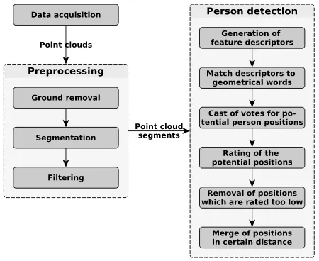
A diagram of the approach is shown in Figure 2. It consists of a preprocessing and the actual detection of persons. The prepro-cessing allows us to reduce the amount of data early on with sev-eral lightweight algorithms. This should increase the ovsev-erall pro-cessing speed. The output of the prepropro-cessing are several point cloud segments which could represent a person. These segments are then classified in the classespersonandno personusing an ISM approach.
Figure 2. Schematic diagram of our approach
3.1 Preprocessing
The preprocessing is divided into the three consecutive steps:
Re-moval of ground,segmentationandfiltering of the segments. Each
of these steps is described in this section.
3.1.1 Ground removal The first step of the preprocessing is the removal of the ground. This serves two purposes. It greatly reduces the amount of data and it enables us to properly perform a segmentation in the next step, since otherwise most segments would be connected by the ground. For the ground removal we first generate a ground grid, which describes the surface of the ground. Afterwards we remove every point which is within a certain distance from this grid.
value of the 0.05 quantile as height value of the cell. The 0.05 quantile is used to deal with outliers inside that cell.
After we have determined a height value for each cell, we have to evaluate which cells actually contain any ground, since there are cells which contain no ground at all. To do that we recursively traverse the grid originating from a start cell. While traversing, it is checked for the current cell which of its neighboring cells could be reached. A cell counts as reachable if the height difference between it and the current cell does not violate a parameter for the maximum steepness of the ground. Every reachable cell will be traversed and used as a current cell later on, until there are no (not already traversed) reachable cells left. Cells which could not be reached while traversing are removed from the ground grid since we assume that they do not contain any ground. For determining the start cell three criteria are used:
1. The height value of the cell should be between the 0.05 and 0.15 quantile of the height values of all cells. This is done to make sure that the start cell contains ground and to deal with potential outlier cells which have a height value below the actual ground.
2. The number of reachable neighboring cells. Cells with a high amount of reachable neighbors are preferred as start cell.
3. The distance to the center of the grid. Cells near the center are preferred.
3.1.2 Segmentation and filtering As soon as the ground is removed, we perform a region growing segmentation based on the Euclidean distance. After this step points which are part of the same object should be part of the same segment. The seg-ments are then filtered based on several criteria which can be de-termined with low computational cost. The purpose of this is to reduce the amount of segments which have to be processed by the computationally more expensive detection process.
The first filter which is applied removes segments with only a small amount of points since such segments do not contain enough information to be successfully classified. The second fil-ter uses the geometrical aspect ratio of the segments to remove segments which are basically long lines. For such segments we can say that they are no person. A third filter removes segments which are either too small or too large to be a person.
3.2 Person detection
For the detection of persons in the resulting segments of the pre-processing we use an ISM approach. Such an approach allows us to work with small amounts of training data (Velizhev et al., 2012). In our opinion it has also great potential in dealing with a low point density and is able to process data fast enough to keep up with the data acquisition speed of a MLS system. These are the challenges which we have mentioned in Section 1.
In this section we first give an overview of our approach and its processing steps while detecting objects in the data. Then we will cover several aspects of the approach in greater detail. Although we currently only detect persons, the approach itself is able to detect various kinds of object classes. The processing steps of our approach are:
1. Generation of a feature descriptor for each point of each seg-ment.
2. Search for the best matching geometrical word in the dic-tionary for each descriptor. For this we use a search index for approximate nearest neighbor searches which is based on the approach presented by Muja and Lowe (2009).
3. Each word of the previous step casts one or more votes for the position of an object of a specific class. This is shown in Figure 3a in a simplified way. Actually every point would have a matching word and cast votes.
4. Rating of the potential object positions for which there are votes. Each vote has a weight in the dictionary. In this step the weight of every potential object position is determined by taking into account the weight of the vote which has voted for the position itself and the weight of votes which have voted for positions for the same object class in the vicinity of the potential position. This step is illustrated in Figure 3b. The size of the dots represents their rating.
5. Removal of all potential object positions which have a weight below a certain threshold (Figure 3c).
6. Merge of the remaining potential object positions for the same class which are in a certain distance from each other (Figure 3d). This acts as a non-maxima suppression and is done by using a region-growing-like method for the poten-tial positions.
7. Output of the resulting object positions as recognized ob-jects.
3.2.1 Feature descriptor The feature descriptor is used to de-scribe local parts of the segments which should be classified and the geometric words in the dictionary. As mentioned in Section 2, there are different strategies for the computing of feature scriptors in ISM approaches. One is to use fewer but more de-scriptive descriptors which are computed for well picked interest points (Knopp et al., 2010). Another one is to use a less descrip-tive but faster to compute descriptor and compute it either for a large amount of randomly picked points or for all points of the processed segment (Velizhev et al., 2012). We have decided to use the second strategy since it can deal better with noise and oc-clusions (Velizhev et al., 2012) which are quite common in point clouds generated by single MLS scans. Hence we use a spin im-age descriptor (Johnson and Hebert, 1999) which we compute for every point of the segments.
3.2.2 Training and structure of the dictionary The training process uses segments that are already classified to generate the dictionary of geometric words which is later used by the detector. Each geometric word consists of a feature descriptor and at least one vote. On the other hand a vote consists of the class for which the vote is a 3D vector to the voted object position and a weight factor which is between 0 and 1.
In the training process a descriptor is computed for each point in each training segment. After that, this descriptor together with a vector from the point to the position (center) of the training seg-ment and the class information of the segseg-ment are used to initial-ize a new geometric word with one vote for the class and position. The weight of this vote is initialized with 1.
(a) Geometric words have casted votes
(b) Potential positions are rated
(c) Threshold is applied (d) Remaining potential positions in a certain radius
merged
Figure 3. Illustration of the main processing step of our person detection
their average descriptor as the descriptor of the merged word. By changing thekparameter of thek-means clustering it is possible to control the size of the resulting dictionary.
After merging, the words will have more than one vote since they inherit all the votes of the original words. These votes are now clustered and merged according to their position vector. This is performed separately for each class for which there are votes. For the clustering of the votes, we use a bottom-up complete linkage hierarchical clustering which we abort if the distance for the next best merge is higher than a threshold. The position vector of the newly merged votes is the average position vector of their original votes. In a final step we recalculate the vote weight for each vote of the merged words:
Wv(wi) =
1 Nv(wi)
(1)
where Wv(wi)= Weight for each vote of wordwi
Nv(wi)= Number of votes of wordwi
This ensures that the total vote weight of each word is 1. This
means that votes of words which only cast one or a few votes have a higher weight than votes of words which cast many dif-ferent votes. Thereby we favor more descriptive words over less descriptive ones.
For the resulting dictionary a search index in the feature space is generated which is later used to find the matching words for fea-ture descriptors. For this search index the approach presented by Muja and Lowe (2009) is utilized. This method allows fast ap-proximate nearest neighbor searches in high-dimensional spaces. It automatically decides between a algorithm based on random-ized kd-trees and one based on hierarchical k-means trees and parameterizes them given a desired precision and weight factors for memory usage and index build time.
3.2.3 Rating of potential object positions As already men-tioned in Section 3.2, the rating of the potential object positions is step four of our detection process and takes place after each geo-metrical word, matched with the segment which is currently been processed, has cast its votes. It serves the purpose of determining which of the potential object positions is the position of an actual object. For this we use the soft voting scheme: It is assumed that a high vote weight lays either at or in the vicinity of an actual ob-ject position. At the beginning of this step each potential position has the weight of the vote, which originally voted for it (Figure 3a).
At first we determine a normalization factor to limit the total weight of all potential positions to 1:
Wnorm= P1
p∈P
Wp
(2)
where Wnorm= Normalization factor Wp= Weight of positionp
P= All potential object positions
Afterwards the weight of each potential position is recalculated by taking into account its original weight, the normalization fac-tor and a fraction of the weight of other potential positions for the same class in its vicinity (Figure 3b). This fraction is influenced by the distance between the two positions using the Gaussian nor-mal distribution. So the new weight is calculated as follows:
Rp=
X
k∈K
Wk·Wnorm·e −Dpk
2
2σ2 (3)
where Rp= Rated weight of positionp
K= All potential positions with same class asp Wk= Weight of positionk
Wnorm= Normalization factor as defined in (2) Dpk= Euclidean distance between positionspandk
σ= Determines the width of the normal distribution
4. EXPERIMENTS
This section describes several experiments which we have per-formed to determine the performance of our approach. The ex-periments cover the influence which the main parameters of the approach have on the runtime and the detection performance. The influence of the used feature descriptor type and its parameters is not examined but we plan to do a comprehensive analysis on that in a future work. At first we will explain our experimental setup and then present and discuss our results.
4.1 Experimental setup
For our experiments we used data which we have acquired with the measurement vehicle ”MODISSA”1. This vehicle is shown in Figure 4. It is equipped with several LiDAR sensors of which we used the two Velodyne HDL-64E mounted on the roof in the front of the vehicle. These sensors are capable of performing 1.3 million measurements per second in a range up to 120 meters. Their vertical field of view is26.9◦
which is divided into 64 scan lines. Since they have a rotating head, their horizontal field of view is360◦
. In our setup they rotated with10 Hzand we con-sidered every rotation as a single scan respectivelypoint cloud. This means every point cloud consists of approximately 130.000 measurements. Since not every measurement is successful, for example if it is in the direction of the sky, the resulting point clouds are usually smaller. The vehicle is also equipped with an inertial measurement unit (IMU) and two GNSS receivers. These are used to compensate for the movement of the vehicle while acquiring data which prevents distortion effects.
Figure 4. Measurement vehicle MODISSA. Equipped with several sensors including four LiDAR
For the experiments we used two different datasets. One is taken on and around the site of the Technical University of Munich in an urban environment2. The second one contains a staged scene with a single person. We used the second dataset mainly for train-ing purposes but parts of that dataset were also used in our evalu-ation. In total we used 100 point clouds for the evaluation, which were part of multiple short sequences in both datasets. In each of these point clouds persons were annotated manually to cre-ate our ground truth. We distinguish between persons which are fully visible in the point clouds and persons which are only partly visible, for example due to occlusions. For the determination of false negative detections we have ignored persons which are only partly visible since it is difficult to decide at which point it should be possible to detect them. Further point clouds were annotated to
1https://www.iosb.fraunhofer.de/servlet/is/42840/
2Data of this measurement campaign can be found at
http://s.fhg.de/mls1
create a dataset to train our detector. The training dataset contains 244 segments which are a person and 387 examples of segments which are not a person. So our training dataset was comparatively small.
To annotate point clouds for the ground truth and the training data we have processed them with our preprocessing (Section 3.1) and then manually classified the segments. Although this method allows us to annotate point clouds fast and easy, it prohibits us from evaluating the quality of the preprocessing itself. For this we plan to do another analysis in the future.
To evaluate the detection performance of our approach we use the indicatorsprecisionandrecallwhich are defined as follows:
P recision= tp
tp+f p (4)
Recall= tp
tp+f n (5)
where tp= True positive detections f p= False positive detections f n= False negative detections
The experiments were conducted on a computer with an Intel Core i7-6900k CPU which has 8 cores and can process 16 threads parallel due to hyper-threading. The computer has64 GB mem-ory which is far more than needed. The implementation of our approach uses parallel processing and is therefore able to profit from the multiple parallel threads of the CPU.
4.2 Results and discussion
This section covers the results of the evaluation of several aspects of our approach.
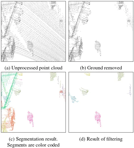
4.2.1 Preprocessing As already mentioned earlier, due to the method we have used to generate our ground truth data we are not able to evaluate our preprocessing quality-wise. But we have analyzed to which extend it fulfills its main purpose of reducing the amount of data to process later on. For this we have ana-lyzed the amount of points which remain after each step of the preprocessing. The results are listed in Table 1. It shows that on average only2.25 %of the original point clouds remain after the preprocessing. This is also shown by the example in Figure 5.
Avg. num. of pts. Percentage
Unprocessed data 97881 100.00 %
Ground removal 53465 54.62 %
Number of points filter 41730 42.63 %
Aspect ratio filter 34412 35.16 %
Size filter 2203 2.25 %
Table 1. Data reduction in preprocessing
4.2.2 Size of the dictionary The size of the dictionary is one of the main influence factors of our approach. As explained in Section 3.2.2, we can control it by changing the value ofkin thek-means clustering. Our training dataset resulted in 263832 geometric words if we do not perform any clustering at all.
(a) Unprocessed point cloud (b) Ground removed
(c) Segmentation result. Segments are color coded
(d) Result of filtering
Figure 5. Processing steps of the preprocessing
needed on average to completely process a single point cloud (preprocessing and detection). This analysis is done by process-ing the evaluation data with dictionaries in different sizes, but the same other parameters. The result of this analysis is shown in Figure 6.
0 50000 100000 150000 200000 250000
Number of words in dictionary 0
200 400 600 800 1000 1200 1400 1600 1800 2000
Average runtime in ms
Figure 6. Influence of the dictionary size on the runtime
The size of the dictionary influences the runtime in two ways: On the one hand, it becomes more difficult to find the matching word for the feature descriptor of a point if the dictionary be-comes more comprehensive. This is the reason why the runtime, on average, slowly increases with a larger dictionary. On the other hand, merging more words together means that a single word on average casts more votes. This is somewhat compensated since we also merge together similar votes of the same word (Section 3.2.2) but is still a factor. It explains why the average runtime be-comes very high when the dictionary is too small for the amount of votes, which is visible on the left of Figure 6.
Figure 7 shows the influence of different dictionary sizes on the
precision and recall of our approach. It is shown that there is a slightly better detection performance if the size of the dictionary increases. Therefore we have a trade-off between the runtime and the detection performance of our approach.
0.0 0.2 0.4 0.6 0.8 1.0
Recall 0.0
0.2 0.4 0.6 0.8 1.0
Precision
10000 words 60000 words 100000 words 200000 words
Figure 7. Precision-Recall curve for different dictionary sizes
4.2.3 Rating of potential object positions As mentioned in Section 3.2.3 the rating of the potential object positions is another crucial step in our detection process. It is influenced by the value of the parameterσin the formula which is used to calculate the rated weight of the potential object positions (cf. Equation 3).
To analyze the influence of theσparameter we have done a simi-lar runtime analysis like with the influence of the dictionary size. For this analysis we have used a dictionary with 60000 geometric words, different values forσand, otherwise, the same parameters. As shown in Figure 8, increasingσ also increases the runtime of the approach. This is to be expected since we consider other potential positions up to a distance of2σwhile rating a single position. Therefore increasingσmeans that we have to consider more positions and have to do more calculations for the rating of a single position. At very high values forσthe curve flattened since we reach a point at which we often consider nearly all po-tential positions of the currently processed segment. In that cases increasingσfurther does not increase the complexity of the rating process anymore.
0.0 0.1 0.2 0.3 0.4 0.5 0.6 0.7 0.8 0.9 1.0
value of σ
0 200 400 600 800 1000 1200 1400 1600 1800 2000
Average runtime in ms
The influence which the parameterσhas on precision and recall of the approach is shown in Figure 9. As with the dictionary size the results show that there is a trade-off between the runtime and the detection performance. It is also shown that a too smallσ greatly decreases the detection performance by only slightly in-creasing the runtime performance. Therefore too smallσ-values are not viable.
Figure 9. Precision-Recall curve for different values forσ
4.2.4 Further analysis of the runtime Right now we are not completely satisfied with the runtime of our approach. As men-tioned earlier we like to be able to process data with approxi-mately the speed of acquisition. Therefore we have analyzed our current approach further to find out which of its components con-sume how much time. For this we have processed our evaluation data with a dictionary of 60000 words, aσof 0.3 for the rating of potential positions. These values are a reasonable compro-mise between the runtime and the detection performance. For this experiment we used 0.17 as threshold for a detection. This parameterization achieves a precision of 0.68 and a recall of 0.76. As before we determined the average runtime per point cloud but this time we break down the runtime for the individual processing steps of the preprocessing and the object detection. The results are shown in Table 2.
Avg. runtime Percentage
Ground removal 55.12 ms 9.29 %
Segmentation 84.35 ms 14.21 %
Filtering 1.42 ms 0.24 %
Miscellaneous 5.81 ms 0.98 %
Preprocessing 146.70 ms 24.72 %
Compute features 21.14 ms 3.56 %
Find words and cast votes 252.85 ms 42.60 %
Rate positions 144.41 ms 24.33 %
Miscellaneous 28.44 ms 4.79 %
Object detection 446.84 ms 75.28 %
Total 593.54 ms
Table 2. Average runtime of each processing step for dictionary of 60000 words andσof 0.3.
The analysis shows that the search in the dictionary is the most time consuming processing step in our approach. The time needed for this step is determined by the parametrization of the search index and the size of the dictionary as well as the com-plexity of the feature descriptor. As mentioned earlier we use the
approach presented by Muja and Lowe (2009) as search index for the dictionary. Until this point we used 0.95 as precision param-eter of that approach. This means that approximately95 %of the searches for the best matching word would result in the actual best matching word. The build time and memory weight we used is 0 since memory usage is currently no concern of us and we only build the index once as part of our training. Reducing the precision of the search index would be a way to increase the run-time performance of the searches in the dictionary. We performed an experiment to analyze the impact which a reduced search in-dex precision has on the runtime and the detection performance of our approach. For this we repeated the runtime experiment with different search index precisions and otherwise the same pa-rameters. The result of this experiment is visible in Figure 10. It is shown that decreasing the precision of the search index greatly reduces the runtime of searches in the dictionary. Until a certain point the influence on the detection performance is minimal. Us-ing a search index precision of 0.5 reduces the average runtime of the dictionary searches to32 ms. The total average runtime in that configuration is approximately370 msand the achieved precision and recall still are approximately 0.68 and 0.76.
0.0 0.1 0.2 0.3 0.4 0.5 0.6 0.7 0.8 0.9
Figure 10. Different desired precisions for the search index of our dictionary and their influence on the detection performance
and the runtime of searches in the dictionary
Since we already have used a nearly optimal dictionary size for the given parameters, the remaining potential for runtime im-provements of the dictionary searches lies in the feature descrip-tor. As mentioned earlier the feature descriptor, so far, was not in the focus of our experiments. Currently we use spin images with 153 bins which therefore are represented by 153 dimensional his-tograms. We think that it is possible to increase the runtime per-formance of the search in the dictionary if we reduce the dimen-sionality of the feature descriptor. Whether that is true and how it will affect the detection performance of our approach remains to be analyzed in future experiments. Of course the overall search time could also be decreased by reducing the amount of feature descriptors which are computed.
achieved by computing feature descriptors for a smaller amount of points. The second one could be achieved by modifying the threshold for the clustering of similar votes of the same word (Section 3.2.2). But the dictionary which we used for this exper-iment has 163194 votes and 60000 words. Therefore on average each word has 2.7 votes which probably could not be reduced much further.
In the preprocessing the segmentation is the most time consum-ing part. Unfortunately region growconsum-ing is not an algorithm which can easily be parallelized. Our implementation uses paralleliza-tion but that comes at the cost that we have to deal with the fact that sometimes the same segment is generated multiple times in different threads. Such cases are detected but it still means that parts of the region growing are unnecessarily done multiple times.
5. CONCLUSION AND FUTURE WORK
We have demonstrated that it is possible to detect persons in the 3D point clouds acquired by a MLS system. Our approach achieves a good runtime and consists of a preprocessing and a detection step which uses implicit shape models. We have per-formed an initial evaluation of the approach on a dataset which was taken in an urban environment. In this evaluation we ex-perimented with different parameters of the approach and have analyzed their influence on the runtime and the detection perfor-mance. For this we have determined precision and recall of the different configurations. As part of an in-depth analysis of the runtime, we used a configuration which offers a good compro-mise between the runtime and detection performance. With this configuration we achieved a runtime of370 ms, a precision of 0.68 and a recall of 0.76.
In future works we plan to perform a more comprehensive eval-uation of our approach which includes the usage of benchmark datasets. We plan to increase the performance of our approach with various measures. One will be to increase the amount of positive and negative training datasets. We assume this will in-crease the overall precision and recall of the approach. Right now the amount of used training datasets is very low which prob-ably causes some problems in the area of generalization. We also plan to evaluate different parameterizations of the spin image de-scriptor which we currently use and to evaluate additional feature descriptors.
Another task will be the in depth evaluation of our preprocessing. As part of this we like to evaluate the removal of the segmen-tation and the subsequent filtering step to work with the unseg-mented point clouds. This will solve problems with under- or over-segmentation of the data and saves the time which is needed for the segmentation. Of course it will also increase the time needed for the actual detection. To add a tracking component to our approach which should help us to increase the performance in both runtime and quality by keeping track of already detected per-sons and to work with multiple sensors at once are also planned for the future.
References
Behley, J., Steinhage, V. and Cremers, A. B., 2013. Laser-based segment classification using a mixture of bag-of-words. In: 2013 IEEE/RSJ International Conference on Intelligent Robots
and Systems, pp. 4195–4200.
Johnson, A. E. and Hebert, M., 1999. Using spin images for ef-ficient object recognition in cluttered 3d scenes. IEEE
Trans-actions on Pattern Analysis and Machine Intelligence21(5),
pp. 433–449.
J¨ungling, K. and Arens, M., 2011. View-invariant person re-identification with an implicit shape model. In:2011 8th IEEE International Conference on Advanced Video and Signal Based
Surveillance (AVSS), pp. 197–202.
Knopp, J., Prasad, M., Willems, G., Timofte, R. and Van Gool, L., 2010. Hough transform and 3d surf for robust three dimen-sional classification. In: Proceedings of the 11th European
Conference on Computer Vision: Part VI, ECCV’10,
Springer-Verlag, Berlin, Heidelberg, pp. 589–602.
Leibe, B., Leonardis, A. and Schiele, B., 2008. Robust object de-tection with interleaved categorization and segmentation.
In-ternational Journal of Computer Vision77(1), pp. 259–289.
Maturana, D. and Scherer, S., 2015. Voxnet: A 3d convolu-tional neural network for real-time object recognition. In:2015 IEEE/RSJ International Conference on Intelligent Robots and
Systems (IROS), pp. 922–928.
Muja, M. and Lowe, D. G., 2009. Fast approximate nearest neigh-bors with automatic algorithm configuration. In:International Conference on Computer Vision Theory and Application
VIS-SAPP’09), INSTICC Press, pp. 331–340.
Navarro-Serment, L. E., Mertz, C. and Hebert, M., 2010. Pedes-trian detection and tracking using three-dimensional ladar data. The International Journal of Robotics Research29(12), pp. 1516–1528.
Premebida, C., Carreira, J., Batista, J. and Nunes, U., 2014. Pedestrian detection combining rgb and dense lidar data. In: 2014 IEEE/RSJ International Conference on Intelligent Robots
and Systems, pp. 4112–4117.
Shotton, J., Fitzgibbon, A., Cook, M., Sharp, T., Finocchio, M., Moore, R., Kipman, A. and Blake, A., 2011. Real-time human pose recognition in parts from a single depth image. In:CVPR, IEEE.
Shotton, J., Girshick, R., Fitzgibbon, A., Sharp, T., Cook, M., Finocchio, M., Moore, R., Kohli, P., Criminisi, A., Kipman, A. and Blake, A., 2013. Efficient human pose estimation from single depth images. IEEE Transactions on Pattern Analysis
and Machine Intelligence35(12), pp. 2821–2840.
Socher, R., Huval, B., Bath, B., Manning, C. D. and Ng, A. Y., 2012. Convolutional-recursive deep learning for 3d object classification. In:Advances in Neural Information Processing
Systems, pp. 656–664.
Spinello, L., Arras, K. O., Triebel, R. and Siegwart, R., 2010. A layered approach to people detection in 3d range data. In: AAAI, Citeseer.
Velizhev, A., Shapovalov, R. and Schindler, K., 2012. Implicit shape models for object detection in 3d point clouds. ISPRS Annals of Photogrammetry, Remote Sensing and Spatial