CHARACTERISTICS OF INDONESIAN HOUSEHOLD’S LIVING EXPENDITURE

(1)

JEJAK

Journal of Economics and Policy

http://journal.unnes.ac.id/nju/index.php/jejak

CHARACTERISTICS OF INDONESIAN HOUSEHOLD’S

LIVING EXPENDITURE

Duddy Roesmara Donna

Gadjah Mada University, Yogyakarta, Indonesia

Permalink/DOI: http://dx.doi.org/10.15294/jejak.v7i1.3596

Received : Februari 2014; Accepted: Maret 2014; Published: September 2014 Abstract

The aim of this study is to estimate and analize the characteristics of Indonesian household expenditure on goods and services, for example food, clothes, household utensils, housing, medical care, education, oil and transportation, gas, electricity and communication. Linear Expenditure System (LES) model and seemingly uncorrelated regression (SUR) estimation method were applied. This study has some conclusions. First, if ones have more incomes, they will proportionally allocate them for housing, oil and transportation, education, food, and medical care. Second, medical care, education and communication are categorized as superior or deluxe commodities. Third, the approximation of minimum living expenditure to survive is Rp 147.236 for a household per week.

Keywords: Living expenditure, Linear Expenditure System (LES), Seemingly Uncorrelated Regression (SUR)

Abstrak

Tujuan dari artikel ini adalah mengestimasi dan menganalisis karakteristik pengeluaran rumah tangga di Indonesia dalam bentuk barang dan jasa, seperti makanan, pakaian, peralatan rumah tangga, perumahan, perawatan medis, pendidikan, transportasi dan bahan bakar, gas, listrik, komunikasi. Model Linear Expenditure System (LES) dan metode estimasi Seemingly Uncorrelated Regression (SUR) digunakan dalam penelitian ini. Penelitian ini menunjukkan beberapa kesimpulan. Pertama, penambahan pendapatan akan dialokasikan secara proporsional untuk perumahan, transportasi dan bahan bakar, pendidikan makanan, perawatan medis. Kedua, perawatan medis, pendidikan, komunikasi adalah termasuk barang atau kebutuhan superior. Ketiga, perkiraan pengeluaran rumah tangga minimum sebesar Rp 147.236 per minggu.

Kata Kunci: pengeluaran hidup, Linear Expenditure System (LES), Seemingly Uncorrelated Regression (SUR)

How to Cite: Donna, Duddy R. (2012). Characteristics of Indonesian Household’s Living Expenditure. JEJAK

Journal of Economics and Policy, 7 (2): 100-202 doi: 10.15294jejak.v7i1.3596

_{Corresponding author :}

Address: Kantor Pusat UGM, Lt. 1, Sayap Selatan, Bulaksumur, Yogyakarta - 55281 E-mail: duddyroes@gmail.com

(2)

101

INTRODUCTION

Identifying the characteristics of li-ving expenditure becomes very important for decision making of policy analysis. Li-ving expenditure is strong related with the demand characteristic of basic need. Elaine (1999) notes that there are 5 factors affecting food decisions made by individual consu-mers i.e. food availability, cultural factors, psychological factors, lifestyle factors and food trends. By assuming unchanged hous-ehold preferences, the change of minimum expenditure can easily found by multiplying the minimum good i by its own price and then summing up them.

However, the current financial crisis seems to have affected consumers’ attitudes in many countries. The economic uncer-tainty and insecurity have led consumers to take decisions minimizing their costs, even for basic needs, such as food quantity and

quality. In a period of inflation and unemp

-loyment, consumers are more likely to chan-ge the composition of their expenditures. (Barda and Sardinou, 2010). Furthermore, the household behaviour of expenditures on food is directly related to the household size. As expected, previous studies have es-timated that there exists a positive relation-ship between the number of members in a household. (Kostakis, 2012)

In evaluating a household’s well-being, one must not be limited to the household’s actual welfare status today, but must also ac-count for the household’s prospects for being well in the future, and being well today does not imply being well tomorrow (Baiyegunhi, LJS, and Fraser, 2010). Secondly, understan-ding vulnerability is also important from an instrumental perspective. Because of the many risks household face, they often expe-rience shocks leading to a wide variability in their endowment and income.

All econometric studies of demand are related to the three basic objectives of econometrics, i.e. (1) structural analysis, (2) forecasting and (3) policy evaluation

(Grif-fiths et al., 1993; Intriligator et al., 1996; Gu

-jarati, 2000). First, the structural analysis

is connected with the use of an estimated

econometric model for the quantitative me-asurement of economic relationships. Many researches of demand focus on some aspects of structural analysis, particularly the esti-mation of the impacts of the change in pri-ces and income on the quantity demanded,

as measured by elasticity. Second,

forecas-ting concerns with the use of an estimated econometric model to predict quantitative values of certain variables outside the samp-le of data actually observed. Many researches of demand are oriented toward forecasting, in particular forecasting quantities, and/or prices of specific commodities in either the

short or the long period. Third, policy

eva-luation is related to the use of an estima-ted econometric model to choose between alternative policies. Researches of demand are sometimes oriented toward policy eva-luation, in particular, the impact of policies (such as taxes and subsidies) that may affect markets for consumer goods. From the es-timated demand function, it is possible to predict the impacts of taxes or subsidies on the quantities demanded, welfare changes, for example (Widodo, 2006).

The idea of standard of living of In-donesian households relates to various ele-ments of household’s livelihood and varies by income. By using Linear Expenditure System (LES), characteristic of living

expen-diture can be explained. It is stated that x_io

represents the minimum good consumed by

household and p_ix_io_{the minimum}

expendi-ture to which the household is committed (subsistence expenditure) (Stone 1954).

This paper aims to analyze the charac-teristics of Indonesian living expenditure and to approximate minimum living expen-diture to survive. In this paper, the groups consist of (1) Food, (2) Clothes, (3) House-hold utensils, (4) Housing, (5) Medical Care, (6) Education, (7) Oil and Transportation, (8) Gas, (9) Electricity and (10)

Communi-cation. The rest of this paper is organized

(3)

Theoretically, a household’s demand for goods and services is a function of prices

and income (by the definition of Marshal

-lian demand function). The problem of the household is to choose quantity of goods and services that maximize its utility func-tion subject to the given budget constraint. Therefore, some changes in income and pri-ces of goods and servipri-ces will directly affect the number of goods and services deman-ded. This section describes a utility func-tion, which derives the linear expenditure system (LES), and shows formulas of elasti-cities under the LES.

In this paper, we assume that Indone-sian households have a utility function follo-wing the more general Cobb-Douglas (CD)

for a simplicity reason1_{. Stone (1954) makes}

the first attempt to estimate an equation system incorporating explicitly the budget constraint, namely the linear expenditure system (LES). Klein and Rubin (1948) for-mulate the LES as the most general linear formulation in prices and income satisfying the budget constraint, homogeneity and the Slutsky symmetry (Mas-Colell et al., 1995) Samuelson (1948) and Geary (1950) derive the LES from the following utility functi-on:

The problem of individual

house-hold is to choose the combination of x_i that

can maximize its utility U(x_i) subject to its

budget constraint. Therefore, the optimal

1 In fact, we can choose the appropriate

utility function by conducting a non-nested test of comparison between two demand systems (See for examples - as they are cited by Katchova and Chern (2004): between the linear and the quadratic expenditure systems (LES and QES) by Polak and Wales (1978), between the QES and the translog demand system by Pollak and Wales (1980), between the translog demand system and the AIDS by Lewbel (1989), between the AIDS and the Rotterdam demand system by Alston and Chalfant (1993), between alternative demand system combining the Rotterdam model and the AIDS by Lee et al. (1994), between

the absolute price Rotterdam model and the first differenced linear approximate AIDS by Kastens

and Brester (1996)).

choice of x_i is obtained as a solution to the

constrained optimization problem as fol-lows:

product operator and x_i is consumption of

commodity i. Then x_io_{and a}

i are the

parame-ters of the utility function. x_io_{is minimum}

quantity of commodity i consumed and

iÎ[1,2,3……..n]. P is a row vector of prices and

X is a column vector of quantity of

commo-dity while M is income

Solving the above optimization

prob-lem, we can find the Marshallian (uncom

-pensated) demand function for each

com-modity x_i as follows:

Where: iÎ(1,2,……..n) jÎ(1,2,……..n)

Since the restriction that the sum of

parameters a_i equals one, 1

sed, Equation (2) simply becomes:

p the linear expenditure system as follows:



Equation (4) shows that the

expendi-ture on good i , denoted as p_ix_i, can be

di-vided into two components. The first com

-ponent is the expenditure on a certain base

amount x_io_{of good i, which is the minimum}

expenditure to which the consumer is

com-mitted (subsistence expenditure), p_ix_io

(Sto-ne, 1954). Samuelson (1948) interprets x_io

as a necessary set of goods resulting in an

informal convention of viewing x_io _as

non-negative quantity.

(4)

103

The restriction of x_io_{to be}

non-nega-tive however is unnecessarily strict. In fact, the utility function is still defined whenever

0

x

i− oi > . Thus, Pollak (1968) argues that

the interpretation of x_io_{as a}_{necessary level}

of consumption is misleading. Allowing x_io _to

be negative provides an additional flexibility in the possibility of price-elastic goods. The usefulness of this generality in price elasti-city depends on the level of aggregation at which the system is treated. The broader is the category of goods, the more probable is the price elastic. Solari (in Howe, 1974:13)

in-terprets negativity of x_io_as_superior_or_deluxe

commodities.

In order to preserve the committed

quantity interpretation of the x_io_{when some}

x_io are negative, Solari (1971) redefines the

quantity p xo

j n

1

j j

∑

= as “augmented

supernu-merary income” (in contrast to the usual interpretation as supernumerary income,

regardless of the signs of the x_io_{). Then, by}

defining n* such that all goods with i£n*

have positive x_io and goods for i>n* are su

-perior with negative x_io_{, Solari interprets}

x p o

j 1 j j

n*

∑

=

as supernumerary income and

x p o

j n

1 j

j

n* ∑

+ =

as fictitious income. The sum of “Solary-supernumerary income” and fictitio -us income equals augmented supernumera-ry income. Although somewhat convoluted, these redefinition allow the interpretation of ‘Solari-supernumerary income’ as expen-diture in excess of the necessary to cover committed quantities. From this analysis can be classified the type of goods services.

If the minimum quantity of good (q_io_{) has}

positive value, it can be classified as basic need goods. On the other hand, if the value is not positive, it means that the good is not basic needs.

The second component is a fraction

a_i of the supernumerary income, defined as

the income above the “subsistence income”

x p o

j n

1

j j

∑

= that is needed to purchase a base

amount of all goods. The sum of coefficients

a_i equals one to simplify the demand

func-tions. The coefficients a_i are referred to as

the marginal budget share, a_i /åa_i. They

indi-cate the proportions in which the incremen-tal income is allocated. From this analysis can be classified the type of goods services.

If the marginal budget share (a_i) has

posi-tive value, it can be classified as no inferior goods. On the other hand, if the value is not positive, it means that the good is inferior.

RESEARCH METHOD

To estimate the coefficients and cons

-tants in the LES model requires data on prices, quantities, and incomes. This paper uses panel secondary data. The source of data refers to Susenas (Survei Sosial Ekono-mi Nasional, National Survey of Social and Economy) that is published by BPS (Badan Pusat Statistik, Statistics Bureau of Indone-sia) in July 2009 and March 2010. The ana-lysis covers 33 provinces in Indonesia. Data of income and quantity are available on Su-senas. Data of price can be estimated by di-vide income with quantity. It is not a good price but a weighted commodity price. The

province average is used to break away diffe

-rent structure of data (July 2009 and March 2010). The unit of data is in household per week.

The estimation of a linear expenditure system (LES) shows certain complications because while it is linear in the variables, it is non-linear in the parameters, involving

the products of a_i and xoi in Equation

sys-tems (3) and (4). There are several approa-ches to estimate the system (Intriligator et al., 1996).

The first approach determines the mi

-nimum quantities xoi based on extraneous

information or prior judgments. Equation system (4) then implies that expenditure on each good in excess of the minimum

ex-penditure

(

px pxo

)

i i i

i − is a linear function of

supernumerary income, so each of the

mar-ginal budget shares (a_i) can be estimated by

applying the usual single-equation simple linear regression methods.

The second approach reverses the first one by determining the marginal budget

shares a_i based on extraneous information

(5)

which estimate a_i from the relationship bet-ween expenditure and income). It then

es-timates the minimum quantities (

x

oi) by

estimating the system in which the expen-diture less the marginal budget shares time

income

(

px xo

)

i i i

i −α is a linear function of all

prices. The total sum of squared errors -over all goods as well all observations- is then

mi-nimized by choice of the xo

i

The third approach is an iterative one,

by using an estimate of a_i conditional on the

x

oi (as in the first approach) and the esti

-mates of the

x

oi conditional on a_i (as in the

second approach) iteratively so as to mini-mize the total sum of squares. The process

would continue, choosing a_i based on

esti-mate

x

oi and choosing

x

o

i based on the last

estimated a_i, until convergence of the sum of

squares is achieved.

The fourth approach selects a_i and

x

oi

simultaneously by setting up a grid of pos-sible values for the 2n-1 parameters (the –1

based on the fact that the sum of a_i tends to

= ) and obtaining that point

on the grid where the total sum of squares over all goods and all observations is mini-mized.

This paper applies the fourth appro-ach. The reason is that when estimating a system of equation seemingly unrelated regression (SUR), the estimation may be iterated. In this case, the initial estimation is done to estimate variance. A new set of re-siduals is generated and used to estimate a new variance-covariance matrix. The matrix is then used to compute a new set of para-meter estimator. The iteration proceeds un-til the parameters converge or unun-til the ma-ximum number of iteration reached. When the random errors follow a multivariate nor-mal distribution these estimators will be the maximum likelihood estimators (Judge et al., 1982).

Rewriting Equation (4) to accom-modate a sample t=1,2,3,…..T and 10 goods yields the following econometric non-linear system:

Where: e_it is error term equation

(good) i at time t.

Given that the covariance matrix

[ ]

=ξ

x is not diagonal matrix, this system can be viewed as a set of non-linear seemingly unrelated regression (SUR) equations. The-re is an added complication, however.

Be-cause M

variables is equal to one of the explanato-ry variables for all t, it can be shown that

(_e₁_t+_e₂_t+...+_e₁_t_o)=0 and hence x is singular,

leading to a breakdown in both estimation procedures. The problem is overcome by estimating only 9 of the ten equations, say the first nine, and using the constraint that

1

maining coefficient a₁₀(Barten, 1977).

The first equations were estimated using the data and the maximum likeli-hood estimation procedure. The nature of the model provides some guides as to what might be good starting values for an

iterati-ve algorithm2_{. Since the constraint the}

mi-nimum observation of expenditure on good

i at time t (x_it) greater than the minimum

expenditure

x

io should be satisfied, the mi

-nimum x_it observation seems a reasonable

starting value for

x

ioin iteration process.

Also the average budget share, ∑

=

the iterating process (Judge et al, 1982). It is

because the estimates of the budget share a_i

will not much differ with the average budget share.

RESULT AND ANALYSIS

Table 1 describes the estimates of the

2 For a detailed explanation about iterative

algorithms, see Griffith et al 1982.

(6)

105

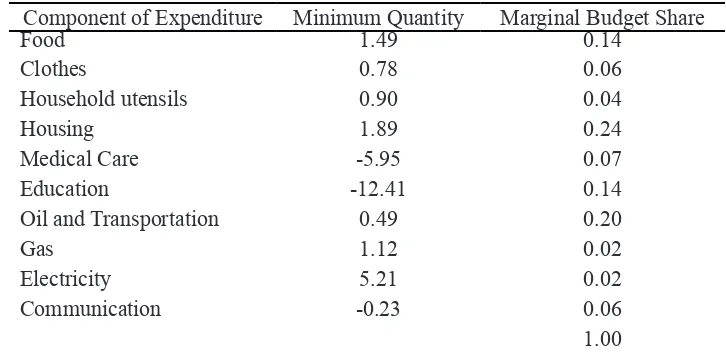
LES for the Indonesian household. There are two components of living expenditure that can be analyzed from LES’s result, i.e. minimum quantity and marginal budget share.

The unit of minimum quantity is in quantity unit. From the value minimum quantity, it can be concluded that food, clothes, household, utensils, housing, oil and transportation, gas, and electricity are basic need commodities (positive value). Baiyegunhi (2010). On the other hand, me-dical care, education, and communicati-on are not basic need commodities (ncommunicati-on positive value) for surviving. In fact, many people can be survival without education and communication expenditure. Because of poverty, many people can’t access

edu-cation and standard medical care. For poor people, standard (formal) medical care can be substituted by traditional medical care. It is cheaper than standard medical care. On the other hand, poor people can access standard medical care and education with several subsidy programs from government, even can be zero cost.

From the value of marginal budget share (positive), it can be concluded that all of commodities are non inferior good. It me-ans that if the income increase will affect the increase of consumption (quantity of good). From the rank of marginal budget share va-lue, it can be concluded that housing, oil and transportation, education, food, and medical care are the most important expen-diture if household get additional income

Table 1. Minimum Quantity and Marginal Budget Share of Indonesian Household

Component of Expenditure Minimum Quantity Marginal Budget Share

Food 1.49 0.14

Clothes 0.78 0.06

Household utensils 0.90 0.04

Housing 1.89 0.24

Medical Care -5.95 0.07

Education -12.41 0.14

Oil and Transportation 0.49 0.20

Gas 1.12 0.02

Electricity 5.21 0.02

Communication -0.23 0.06

1.00

Source: Susenas, July 2009 and March 2010, BPS, authors’ calculation

Table 2. Minimum Household’s Living Expenditure

Component of Expenditure Minimum Expenditure Share

Food 99,314 67.43%

Clothes 3,110 2.11%

Household utensils 4,137 2.81%

Housing 15,725 10.68%

Medical Care 0 0.00%

Education 0 0.00%

Oil and Transportation 10,658 7.24%

Gas 9,653 6.55%

Electricity 4,692 3.19%

Communication 0 0.00%

Total 147,289 100.00%

(7)

(above supernumerary income).

Minimum living expenditure can be estimated from the multiplication of mini-mum quantity and weighted price of com-modity except medical care, education, and communication (These are not basic need goods).

Tabel 2 describes the detail of household’s minimum living expenditures (in Rupiah per household per week). Based on the value, the rank of component expen-diture are food, housing, oil and transporta-tion, gas, electricity, household utensils, and

clothes. More than 50 percent of minimum expenditure is allocated for food. Total of minimum living expenditure is Rp 147.289 for a household per week.

CONCLUSIONS

This paper analyses estimates and analyses the characteristics of Indonesi-an household’s living expenditures. Linear Expenditure System (LES) model and see mingly uncorrelated regression (SUR) esti-mation method is applied on this analysis.

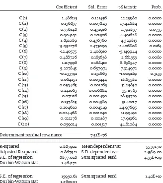
Appendix: Estimation Result of the LES System: SUR0910

Estimation Method: Seemingly Unrelated Regression Date: 01/18/13 Time: 20:13

Sample: 1 66

Included observations: 66

Total system (balanced) observations 660

One-step final coefficients from consistent one-step weighting matrix

Convergence not achieved after: 1 weight matrix, 6 total coef iterations

Coefficient Std. Error t-Statistic Prob.

C(1) 1.486113 0.121456 12.23580 0.0000

C(11) 0.136837 0.007843 17.44684 0.0000

C(2) 0.776148 0.432916 1.792837 0.0735

C(3) 0.904192 0.201306 4.491628 0.0000

C(4) 1.891089 0.436760 4.329813 0.0000

C(5) -5.952276 2.473099 -2.406808 0.0164

C(6) -12.40575 2.408910 -5.149944 0.0000

C(7) 0.488726 0.183638 2.661353 0.0080

C(8) 1.117996 0.168410 6.638547 0.0000

C(9) 5.207845 0.657974 7.914972 0.0000

C(10) -0.233791 0.231663 -1.009189 0.3133

C(12) 0.064251 0.003444 18.65582 0.0000

C(13) 0.039465 0.001263 31.25830 0.0000

C(14) 0.241063 0.006864 35.11763 0.0000

C(15) 0.071116 0.002490 28.55729 0.0000

C(16) 0.137825 0.004389 31.40017 0.0000

C(17) 0.204620 0.004549 44.97695 0.0000

C(18) 0.024468 0.002040 11.99492 0.0000

C(19) 0.021278 0.001187 17.91962 0.0000

C(20) 0.059014 0.001317 44.81084 0.0000

Determinant residual covariance 7.51E+76

R-squared 0.887902 Mean dependent var 55371.70

Adjusted R-squared 0.867521 S.D. dependent var 24389.00 S.E. of regression 8877.028 Sum squared resid 4.33E+09 Durbin-Watson stat 1.464172

(8)

107

Food, clothes, household, utensils, housing, oil and transportation, gas, and electricity are basic need commodities. Me-dical care, education, and communication are not basic need commodities. All of the commodities are non inferior commodities. Increases in income (above supernumera-ry income) will be proportionally allocated more for Housing, Oil and transportation,

Education, Food, and Medical care. Second,

Medical care , Education, and Communi-cation are superior or deluxe commodities. The approximation of minimum living ex-penditure to survive is Rp 147.236 for a hous-ehold per week with the dominant propor-tion if food.

REFERENCES

c

Baiyegunhi., LJS., and Fraser. (2010). Determinants of Household Poverty Dinamics in Rural Regions of the Eastern Cape Province, South Africa. Barda, C., & E. Sardianou. (2010). Analysing

consum-ers’ ‘activism’ in response to rising prices, In-ternational Journal of Consumer Studies, 34, 133-139.

Barten, A.P. (1977).The system of consumer demand function approach: a review. Econometrica, 45:23-51.

Deaton A.S., and J. Muellbauer. (1980). Economic and Consumer Behaviour. Cambridge: Cambridge University Press.

Deaton, A.S. (1986). Demand analysis. In Z. Griliches and M.D. Intriligator, Ed, Handbook of Econo-metrics, Vol. 2. Amsterdam: North-Holland Publishing Company.

Elaine, H. (1999).Factors affecting food decisions

made by individual consumers. Food Policy.

Equation: Q6*P6=C(6)*P6+C(16)*(M-P1*C(1)-P2*C(2)-P3*C(3)-P4*C(4)-P5 *C(5)-P6*C(6)-P7*C(7)-P8*C(8)-P9*C(9)-P10*C(10))

Observations: 66

Adjusted R-squared 0.665036 S.D. dependent var 49479.63

S.E. of regression 28636.88 Sum squared resid 4.51E+10 Durbin-Watson stat 1.812997

Observations: 66

(9)

Vol. 24: 287-94.

Geary, R.C. (1950). A note on a constant utility index of the cost of living. Review of Economic Studies. XVIII (I), No. 45: 65-66.

Gujarati, Damodar. (2000). Basic Econometrics. Fourth Edition. McGraw Hill.

Griffiths, W., R.C. Hill., and G.G. Judge. (1993). Learn-ing and PracticLearn-ing Econometrics. Canada: John Wiley and Sons, Inc.

Goldberger, A., and T. Gamaletsos. (1970). A Cross-country comparison of consumer expenditure patterns. European Economic Review, 1:357-400.

Howe, H. (1974). Estimation of the Linear and Qua-dratic Expenditure Systems: a Cross-section Case for Colombia. University Microfilm Inter -national, Ann Arbor, Michigan, USA, London, England.

Intriligator, M.D . et al. (1996). Econometric Models, Techniques, and Applications, Second Edition. Prentice–Hall Inc, Upper Saddle River, NJ 07458.

Judge, G.G. et al. (1982). Introduction to the Theory and Practice of Econometrics. . Canada: John Wiley and Sons, Inc.

Katchova, A.L., and W.S. Chern. (2004). Comparison of quadratic expenditure system and almost ideal demand system based on empirical data. International Journal of Applied Economics, 1(1) September: 55-64.

Klein, L.R., and H. Rubin. (1948). A constant utility index of the cost of living. Review of Economic Studies. XV(2). No. 38: 84-87.

Kostakis, Ioannis. (2012). The Determinants of House-holds’ Food Consumption in Greece.

Interna-tional of Food and Agricultural Economics Vol. 2 No. 2 pp. 17-28.

Mas-Colell, A., M.D. Whinston., and J.R.Green. (1995). Microeconomic Theory. New York: Ox-ford University Press.

Pollak, R.A. (1968). Additive utility function and lin-ear Engel curves. Discussion Paper. No 53, De-partment of Economics, University of Pennsyl-vania, revised Feb.

Samuelson, P.A. (1948). Some implication of linear-ity. Review of Economic Studies. XV (2). No. 38: 88-90.

Samuelson, P.A., and W.D. Nordhaus. (2001). Econom-ics. Seventh Edition. McGraw-Hill, New York. Solari, L. (1971). Théorie des Choix et Fonctions de

Consommation Semi-Agrégées: Modéles Sta-tiques. Genéve: Librairie Droz: 59-63.

Stone, R. (1954). Linear expenditure system and de-mand analysis: an application to the pattern of Britissh deman. Economic Journal, 64:511-27. Susenas Survey. (2009-2010). Website https://www.

bps.go.id diakses pada tanggal 11 Januari 2012 The Statistics Bureau of Indonesia (Badan Pusat

Statistik). (2009). National Survey of Social and Economy (Survei Sosial Ekonomi Nasion-al). Indonesia

Widodo, T. (2006). Demand estimation and house-hold’s welfare measurement: case studies on Japan Indonesia. HUE Journal of Economics and Business 2 (2): 103-136.