Even if you never leave your home town, you are an active participant in a global economy.When you go to the grocery store, for instance, you might choose be-tween apples grown locally and grapes grown in Chile. When you make a de-posit into your local bank, the bank might lend those funds to your next-door neighbor or to a Japanese company building a factory outside Tokyo. Because our economy is integrated with many others around the world, consumers have more goods and services from which to choose, and savers have more opportuni-ties to invest their wealth.
In previous chapters we simplified our analysis by assuming a closed economy. In actuality, however, most economies are open: they export goods and services abroad, they import goods and services from abroad, and they borrow and lend in world financial markets. Figure 5-1 gives some sense of the importance of these international interactions by showing imports and exports as a percentage of GDP for seven major industrial countries. As the figure shows, imports and exports in the United States are more than 10 percent of GDP. Trade is even more important for many other countries—in Canada and the United King-dom, for instance, imports and exports are about a third of GDP. In these coun-tries, international trade is central to analyzing economic developments and formulating economic policies.
This chapter begins our study of open-economy macroeconomics. We begin in Section 5-1 with questions of measurement. To understand how the open economy works, we must understand the key macroeconomic variables that measure the interactions among countries. Accounting identities reveal a key in-sight: the flow of goods and services across national borders is always matched by an equivalent flow of funds to finance capital accumulation.
In Section 5-2 we examine the determinants of these international flows. We develop a model of the small open economy that corresponds to our model of the closed economy in Chapter 3. The model shows the factors that determine whether a country is a borrower or a lender in world markets, and how policies at home and abroad affect the flows of capital and goods.
5
The Open Economy
C H A P T E R
No nation was ever ruined by trade.
— Benjamin Franklin F I V E
User JOEWA:Job EFF01460:6264_ch05:Pg 115:19203#/eps at 100%
*19203*
Wed, Feb 13, 2002 9:26 AM In Section 5-3 we extend the model to discuss the prices at which a countrymakes exchanges in world markets. We examine what determines the price of domestic goods relative to foreign goods.We also examine what determines the rate at which the domestic currency trades for foreign currencies. Our model shows how protectionist trade policies—policies designed to protect domestic industries from foreign competition—influence the amount of international trade and the exchange rate.
5-l
The International Flows of Capital
and Goods
The key macroeconomic difference between open and closed economies is that, in an open economy, a country’s spending in any given year need not equal its output of goods and services. A country can spend more than it pro-duces by borrowing from abroad, or it can spend less than it propro-duces and lend the difference to foreigners. To understand this more fully, let’s take another look at national income accounting, which we first discussed in Chapter 2.
f i g u r e 5 - 1
Percentage of GDP
40 35 30 25 20 15 10 5 0
Canada France Germany Italy Japan U.K. U.S. Imports Exports
Imports and Exports as a Percentage of Output: 2000 While international trade is important for the United States, it is even more vital for other countries.
The Role of Net Exports
Consider the expenditure on an economy’s output of goods and services. In a closed economy, all output is sold domestically, and expenditure is divided into three components: consumption, investment, and government purchases. In an open economy, some output is sold domestically and some is exported to be sold abroad. We can divide expenditure on an open economy’s output Y into four components:
➤ Cd, consumption of domestic goods and services,
➤ Id, investment in domestic goods and services,
➤ Gd, government purchases of domestic goods and services,
➤ EX, exports of domestic goods and services.
The division of expenditure into these components is expressed in the identity
Y=Cd+Id+Gd+EX.
The sum of the first three terms,Cd+Id+Gd, is domestic spending on domes-tic goods and services. The fourth term,EX, is foreign spending on domestic goods and services.
We now want to make this identity more useful.To do this, note that domestic spending on all goods and services is the sum of domestic spending on domestic goods and services and on foreign goods and services. Hence, total consumption C equals consumption of domestic goods and services Cd plus consumption of foreign goods and services Cf; total investment I equals investment in domestic goods and services Id plus investment in foreign goods and services If; and total government purchases G equals government purchases of domestic goods and services Gdplus government purchases of foreign goods and services Gf.Thus,
C=Cd
+Cf,
I=Id+If, G=Gd
+Gf.
We substitute these three equations into the identity above:
Y=(C−Cf) +(I−If) +(G−Gf) +EX.
We can rearrange to obtain
Y=C+I+G+EX−(Cf+If+Gf).
The sum of domestic spending on foreign goods and services (Cf+If+Gf) is expenditure on imports (IM). We can thus write the national income accounts identity as
Y=C+I+G+EX−IM.
User JOEWA:Job EFF01460:6264_ch05:Pg 117:19205#/eps at 100%
*19205*
Wed, Feb 13, 2002 9:26 AM output, this equation subtracts spending on imports. Defining net exports tobe exports minus imports (NX=EX−IM), the identity becomes
Y=C+I+G+NX.
This equation states that expenditure on domestic output is the sum of con-sumption, investment, government purchases, and net exports. This is the most common form of the national income accounts identity; it should be familiar from Chapter 2.
The national income accounts identity shows how domestic output, domestic spending, and net exports are related. In particular,
NX= Y −(C+I+G)
Net Exports =Output −Domestic Spending.
This equation shows that in an open economy, domestic spending need not equal the output of goods and services.If output exceeds domestic spending, we export the difference: net exports are positive. If output falls short of domestic spending, we import the difference: net exports are negative.
International Capital Flows and the Trade Balance
In an open economy, as in the closed economy we discussed in Chapter 3,fi nan-cial markets and goods markets are closely related. To see the relationship, we must rewrite the national income accounts identity in terms of saving and invest-ment. Begin with the identity
Y=C+I+G+NX.
Subtract Cand Gfrom both sides to obtain
Y−C−G=I+NX.
Recall from Chapter 3 that Y− C− Gis national saving S, the sum of private saving,Y−T−C, and public saving,T−G.Therefore,
S=I+NX.
Subtracting Ifrom both sides of the equation, we can write the national income accounts identity as
S−I=NX.
This form of the national income accounts identity shows that an economy’s net exports must always equal the difference between its saving and its investment.
The left-hand side of the identity is the difference between domestic saving and domestic investment,S−I, which we’ll call net capital outflow. (It’s some-times called net foreign investment.) If net capital outflow is positive, our saving exceeds our investment, and we are lending the excess to foreigners. If the net capital outflow is negative, our investment exceeds our saving, and we are financ-ing this extra investment by borrowfinanc-ing from abroad. Thus, net capital outflow equals the amount that domestic residents are lending abroad minus the amount that foreigners are lending to us. It reflects the international flow of funds to fi-nance capital accumulation.
The national income accounts identity shows that net capital outflow always equals the trade balance.That is,
Net Capital Outflow =Trade Balance
S−I = NX.
If S−Iand NX are positive, we have a trade surplus. In this case, we are net lenders in world financial markets, and we are exporting more goods than we are importing. If S −I and NX are negative, we have a trade deficit. In this case, we are net borrowers in world financial markets, and we are importing more goods than we are exporting. If S − I and NX are exactly zero, we are said to have balanced tradebecause the value of imports equals the value of exports.
The national income accounts identity shows that the international flow of funds to fi -nance capital accumulation and the international flow of goods and services are two sides of the same coin. On the one hand, if our saving exceeds our investment, the saving that is not invested domestically is used to make loans to foreigners. Foreigners require these loans because we are providing them with more goods and services than they are providing us.That is, we are running a trade surplus. On the other hand, if our investment exceeds our saving, the extra investment must be fi-nanced by borrowing from abroad. These foreign loans enable us to import more
This table shows the three outcomes that an open economy can experience.
Trade Surplus Balanced Trade Trade Deficit
Exports >Imports Exports =Imports Exports <Imports Net Exports >0 Net Exports =0 Net Exports <0 Y>C+I+G Y=C+I+G Y<C+I+G Savings >Investment Saving =Investment Saving <Investment Net Capital Outflow >0 Net Capital Outflow =0 Net Capital Outflow <0
User JOEWA:Job EFF01460:6264_ch05:Pg 119:26240#/eps at 100%
*26240*
Wed, Feb 13, 2002 9:26 AMgoods and services than we export.That is, we are running a trade deficit.Table 5-1 summarizes these lessons.
Note that the international flow of capital can take many forms. It is easiest to assume—as we have done so far—that when we run a trade deficit, foreigners make loans to us.This happens, for example, when the Japanese buy the debt is-sued by U.S. corporations or by the U.S. government. But the flow of capital can also take the form of foreigners buying domestic assets, such as when a citizen of Germany buys stock from an American on the New York Stock Exchange. Whether foreigners are buying domestically issued debt or domestically owned assets, they are obtaining a claim to the future returns to domestic capital. In both cases, foreigners end up owning some of the domestic capital stock.
FYI
The equality of net exports and net capital outflow is an identity: it must hold by the way the numbers are added up. But it is easy to miss the intuition behind this important relationship. The best way to understand it is to consider an example.
Imagine that Bill Gates sells a copy of the Windows operating system to a Japanese con-sumer for 5,000 yen. Because Mr. Gates is a U.S. resident, the sale represents an export of the United States. Other things equal, U.S. net ex-ports rise. What else happens to make the iden-tity hold? It depends on what Mr. Gates does with the 5,000 yen.
Suppose Mr. Gates decides to stuff the 5,000 yen in his mattress. In this case, Mr. Gates has al-located some of his saving to an investment in the Japanese economy (in the form of the Japan-ese currency) rather than to an investment in the U.S. economy. Thus, U.S. saving exceeds U.S. in-vestment. The rise in U.S. net exports is matched by a rise in the U.S. net capital outflow.
If Mr. Gates wants to invest in Japan, however, he is unlikely to make currency his asset of choice. He might use the 5,000 yen to buy some stock in, say, the Sony Corporation, or he might buy a bond issued by the Japanese government. In either case, some of U.S. saving is flowing abroad. Once again, the U.S. net capital outflow exactly balances U.S. net exports.
International Flows of Goods and Capital:
An Example
The opposite situation occurs in Japan. When the Japanese consumer buys a copy of the Win-dows operating system, Japan’s purchases of goods and services (C+I+G) rise, but there is no change in what Japan has produced (Y). The transaction reduces Japan’s saving (S=Y−C−G) for a given level of investment (I). While the U.S. experiences a net capital outflow, Japan experi-ences a net capital inflow.
Now let’s change the example. Suppose that instead of investing his 5,000 yen in a Japanese asset, Mr. Gates uses it to buy something made in Japan, such as a Sony Walkman. In this case, imports into the United State rise. Together, the Windows export and the Walkman import repre-sent balanced trade between Japan and the United States. Because exports and imports rise equally, net exports and net capital outflow are both unchanged.
5-2
Saving and Investment in a
Small Open Economy
So far in our discussion of the international flows of goods and capital, we have merely rearranged accounting identities. That is, we have defined some of the variables that measure transactions in an open economy, and we have shown the links among these variables that follow from their definitions. Our next step is to develop a model that explains the behavior of these variables. We can then use the model to answer questions such as how the trade balance responds to changes in policy.
Capital Mobility and the World Interest Rate
In a moment we present a model of the international flows of capital and goods. Because the trade balance equals the net capital outflow, which in turn equals saving minus investment, our model focuses on saving and investment. To de-velop this model, we use some elements that should be familiar from Chapter 3, but in contrast to the Chapter 3 model, we do not assume that the real interest rate equilibrates saving and investment. Instead, we allow the economy to run a trade deficit and borrow from other countries, or to run a trade surplus and lend to other countries.
If the real interest rate does not adjust to equilibrate saving and investment in this model, what does determine the real interest rate? We answer this question
here by considering the simple case of a small open economy with perfect capital mobility. By “small’’we mean that this economy is a small part of the world market and thus, by itself, can have only a negligible effect on the world interest rate. By “perfect capital mobility’’we mean that residents of the country have full access to world financial markets. In particular, the government does not impede international borrowing or lending.
Because of this assumption of perfect capital mobility, the interest rate in our small open economy,r, must equal the world interest rater*, the real interest
rate prevailing in world financial markets:
r=r*.
Residents of the small open economy need never borrow at any interest rate above r*, because they can always get a loan at r*from abroad. Similarly, residents
of this economy need never lend at any interest rate below r* because they can
always earn r*by lending abroad.Thus, the world interest rate determines the
in-terest rate in our small open economy.
User JOEWA:Job EFF01460:6264_ch05:Pg 121:26242#/eps at 100%
*26242*
Wed, Feb 13, 2002 9:26 AMit has a negligible effect on world saving and world investment. Hence, our small open economy takes the world interest rate as exogenously given.
The Model
To build the model of the small open economy, we take three assumptions from Chapter 3:
➤ The economy’s output Yis fixed by the factors of production and the
pro-duction function.We write this as
Y=Y
_
=F(K
_
,L_).
➤ Consumption Cis positively related to disposable income Y−T. We write
the consumption function as
C=C(Y−T).
➤ Investment Iis negatively related to the real interest rate r. We write the
investment function as
I=I(r).
These are the three key parts of our model. If you do not understand these rela-tionships, review Chapter 3 before continuing.
We can now return to the accounting identity and write it as
NX=(Y−C−G) −I
NX=S−I.
Substituting our three assumptions from Chapter 3 and the condition that the interest rate equals the world interest rate, we obtain
NX=[Y
_
−C(Y
_
−T) −G] −I(r*)
= S
_
−I(r*).
This equation shows what determines saving Sand investment I—and thus the
trade balance NX. Remember that saving depends on fiscal policy: lower
govern-ment purchases Gor higher taxes Traise national saving. Investment depends on
the world real interest rate r*: high interest rates make some investment projects
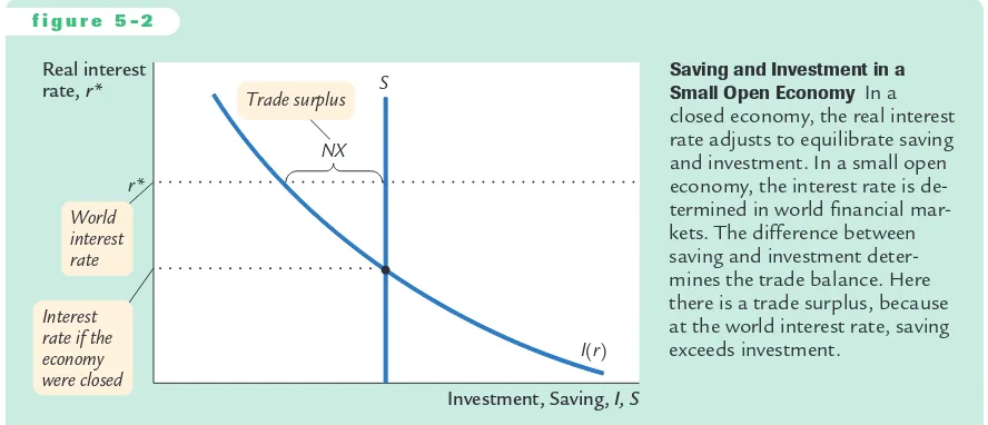
unprofitable.Therefore, the trade balance depends on these variables as well. In Chapter 3 we graphed saving and investment as in Figure 5-2. In the closed economy studied in that chapter, the real interest rate adjusts to equilibrate saving and investment—that is, the real interest rate is found where the saving and in-vestment curves cross. In the small open economy, however, the real interest rate
equals the world real interest rate.The trade balance is determined by the difference
be-tween saving and investment at the world interest rate.
easy to understand.When saving falls short of investment, investors borrow from abroad; when saving exceeds investment, the excess is lent to other countries. But what causes those who import and export to behave in a way that ensures that the international flow of goods exactly balances this international flow of capital? For now we leave this question unanswered, but we return to it in Section 5-3 when we discuss the determination of exchange rates.
How Policies Influence the Trade Balance
Suppose that the economy begins in a position of balanced trade. That is, at the world interest rate, investment Iequals saving S, and net exports NXequal zero. Let’s use our model to predict the effects of government policies at home and abroad.
Fiscal Policy at Home Consider first what happens to the small open
econ-omy if the government expands domestic spending by increasing government purchases. The increase in Greduces national saving, because S = Y − C − G. With an unchanged world real interest rate, investment remains the same.There-fore, saving falls below investment, and some investment must now be financed by borrowing from abroad. Because NX=S−I, the fall in Simplies a fall in NX. The economy now runs a trade deficit.
The same logic applies to a decrease in taxes.A tax cut lowers T, raises dispos-able income Y− T, stimulates consumption, and reduces national saving. (Even though some of the tax cut finds its way into private saving, public saving falls by the full amount of the tax cut; in total, saving falls.) Because NX=S−I, the re-duction in national saving in turn lowers NX.
Figure 5-3 illustrates these effects. A fiscal-policy change that increases private consumption Cor public consumption Greduces national saving (Y− C−G) and, therefore, shifts the vertical line that represents saving from S1to S2. Because NX is the distance between the saving schedule and the investment schedule at the world interest rate, this shift reduces NX.Hence, starting from balanced trade, a change in fiscal policy that reduces national saving leads to a trade deficit.
f i g u r e 5 - 2
Real interest rate, r*
r*
NX S
Investment, Saving, I, S
I(r)
World interest rate
Trade surplus
Interest rate if the economy were closed
User JOEWA:Job EFF01460:6264_ch05:Pg 123:26248#/eps at 100%
*26248*
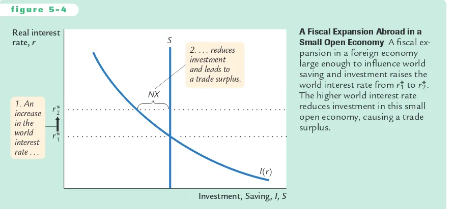
Wed, Feb 13, 2002 9:26 AM Fiscal Policy Abroad Consider now what happens to a small open economywhen foreign governments increase their government purchases. If these foreign countries are a small part of the world economy, then their fiscal change has a negligible impact on other countries. But if these foreign countries are a large part of the world economy, their increase in government purchases reduces world saving and causes the world interest rate to rise.
The increase in the world interest rate raises the cost of borrowing and, thus, reduces investment in our small open economy. Because there has been no change in domestic saving, saving Snow exceeds investment I, and some of our
saving begins to flow abroad. Since NX=S−I, the reduction in Imust also
in-crease NX. Hence, reduced saving abroad leads to a trade surplus at home.
Figure 5-4 illustrates how a small open economy starting from balanced trade responds to a foreign fiscal expansion. Because the policy change is occurring
f i g u r e 5 - 3
Real interest rate, r
r*
NX S1
Investment, Saving, I, S
I(r) S2 2. . . . but when a
fiscal expansion reduces saving . . .
1. This economy begins with balanced trade, . . .
3. . . . a trade deficit results.
A Fiscal Expansion at Home in a Small Open Economy An increase in government purchases or a re-duction in taxes reduces national saving and thus shifts the saving schedule to the left, from S1to S2. The result is a trade deficit.
f i g u r e 5 - 4
Real interest rate, r
r*2
r*1
NX S
Investment, Saving, I, S
I(r)
1. An increase in the world interest rate . . .
2. . . . reduces investment and leads to a trade surplus.
abroad, the domestic saving and investment schedules remain the same.The only change is an increase in the world interest rate from r*1to r*2.The trade balance is the difference between the saving and investment schedules; because saving ex-ceeds investment at r*2, there is a trade surplus.Hence, an increase in the world inter-est rate due to a fiscal expansion abroad leads to a trade surplus.
Shifts in Investment Demand Consider what happens to our small open economy if its investment schedule shifts outward—that is, if the demand for in-vestment goods at every interest rate increases.This shift would occur if, for ex-ample, the government changed the tax laws to encourage investment by providing an investment tax credit. Figure 5-5 illustrates the impact of a shift in the investment schedule.At a given world interest rate, investment is now higher. Because saving is unchanged, some investment must now be financed by bor-rowing from abroad, which means the net capital outflow is negative. Put differ-ently, because NX= S−I, the increase in I implies a decrease in NX.Hence, an outward shift in the investment schedule causes a trade deficit.
f i g u r e 5 - 5
Real interest rate, r
r*
NX S
Investment, Saving, I, S
I(r) 2
I(r) 1
1. An increase in investment demand . . .
2. . . . leads to a trade deficit.
A Shift in the Investment Schedule in a Small Open Economy An outward shift in the investment schedule from I(r)1to I(r)2increases the amount of in-vestment at the world interest rate r*. As a result, investment now exceeds saving, which means the economy is borrowing from abroad and running a trade deficit.
Evaluating Economic Policy
User JOEWA:Job EFF01460:6264_ch05:Pg 125:26250#/eps at 100%
*26250*
Wed, Feb 13, 2002 9:27 AM Our analysis of the open economy has been positive, not normative. That is,our analysis of how economic policies influence the international flows of capi-tal and goods has not told us whether these policies are desirable. Evaluating eco-nomic policies and their impact on the open economy is a frequent topic of debate among economists and policymakers.
When a country runs a trade deficit, policymakers must confront the question of whether it represents a national problem. Most economists view a trade deficit not as a problem in itself, but perhaps as a symptom of a problem. A trade deficit could be a reflection of low saving. In a closed economy, low saving leads to low investment and a smaller future capital stock. In an open economy, low saving leads to a trade deficit and a growing foreign debt, which eventually must be re-paid. In both cases, high current consumption leads to lower future consump-tion, implying that future generations bear the burden of low national saving.
Yet trade deficits are not always a reflection of economic malady.When poor rural economies develop into modern industrial economies, they sometimes fi -nance their high levels of investment with foreign borrowing. In these cases, trade deficits are a sign of economic development. For example, South Korea ran large trade deficits throughout the 1970s, and it became one of the success stories of economic growth.The lesson is that one cannot judge economic performance from the trade balance alone. Instead, one must look at the underlying causes of the international flows.
C A S E S T U D Y
The U.S. Trade Deficit
During the 1980s and 1990s, the United States ran large trade deficits. Panel (a) of Figure 5-6 documents this experience by showing net exports as a percentage of GDP.The exact size of the trade deficit fluctuated over time, but it was large throughout these two decades. In 2000, the trade deficit was $371 billion, or 3.7 percent of GDP. As accounting identities require, this trade deficit had to be fi -nanced by borrowing from abroad (or, equivalently, by selling U.S. assets abroad). During this period, the United States went from being the world’s largest credi-tor to the world’s largest debtor.
What caused the U.S. trade deficit? There is no single explanation. But to un-derstand some of the forces at work, it helps to look at national saving and do-mestic investment, as shown in panel (b) of the figure. Keep in mind that the trade deficit is the difference between saving and investment.
f i g u r e 5 - 6
Percentage of GDP
Investment
Saving
2
1
0
21
22
23
24
25 Surplus
Deficit
1960 1965
Year
1970 1975 1980 1985 1990 1995 2000
Percentage of GDP
1960
Year
20
19
18
17
16
15
14
13
12
11
10
(b) U.S. Saving and Investment (a) The U.S. Trade Balance
1965 1970 1975 1980 1985 1990 1995 2000
Trade balance
The Trade Balance, Saving, and Investment: The U.S. Experience Panel (a) shows the trade balance as a percentage of GDP. Positive numbers represent a surplus, and negative numbers represent a deficit. Panel (b) shows national saving and investment as a percentage of GDP since 1960. The trade balance equals saving minus investment.
User JOEWA:Job EFF01460:6264_ch05:Pg 127:26252#/eps at 100%
*26252*
Wed, Feb 13, 2002 9:27 AM5-3
Exchange Rates
Having examined the international flows of capital and of goods and services, we now extend the analysis by considering the prices that apply to these transac-tions.The exchange rate between two countries is the price at which residents of those countries trade with each other. In this section we first examine precisely what the exchange rate measures, and we then discuss how exchange rates are determined.
Nominal and Real Exchange Rates
Economists distinguish between two exchange rates: the nominal exchange rate and the real exchange rate. Let’s discuss each in turn and see how they are related.
The Nominal Exchange Rate The nominal exchange rate is the relative price of the currency of two countries. For example, if the exchange rate be-tween the U.S. dollar and the Japanese yen is 120 yen per dollar, then you can ex-change one dollar for 120 yen in world markets for foreign currency. A Japanese who wants to obtain dollars would pay 120 yen for each dollar he bought. An American who wants to obtain yen would get 120 yen for each dollar he paid. When people refer to “the exchange rate’’between two countries, they usually mean the nominal exchange rate.
saving, thereby causing a trade deficit. And, in fact, that is exactly what happened. Because the government budget and trade balance went into deficit at roughly the same time, these shortfalls were called the twin deficits.
Things started to change in the 1990s, when the U.S. federal government got its fiscal house in order. The first President Bush and President Clinton both signed tax increases, while Congress kept a lid on spending. In addition to these policy changes, rapid productivity growth in the late 1990s raised in-comes and, thus, further increased tax revenue.These developments moved the U.S. federal budget from deficit to surplus, which in turn caused national sav-ing to rise.
In contrast to what our model predicts, the increase in national saving did not coincide with a shrinking trade deficit, because domestic investment rose at the same time. The likely explanation is that the boom in information technology caused an expansionary shift in the U.S. investment function. Even though fiscal policy was pushing the trade deficit toward surplus, the investment boom was an even stronger force pushing the trade balance toward deficit.
FYI
You can find nominal exchange rates reported daily in many newspapers. Here’s how they are reported in the Wall Street Journal.
Notice that each exchange rate is reported in two ways. On this Thursday, 1 dollar bought 116.29 yen, and 1 yen bought 0.008599 dollars. We can say the exchange rate is 116.29 yen per dollar, or we can say the exchange rate is 0.008599 dollars per yen. Because 0.008599 equals 1/116.29, these two ways of expressing
How Newspapers Report the Exchange Rate
the exchange rate are equivalent. This book al-ways expresses the exchange rate in units of for-eign currency per dollar.
The exchange rate on this Thursday of 116.29 yen per dollar was down from 117.67 yen per dol-lar on Wednesday. Such a fall in the exchange rate is called a depreciationof the dollar; a rise in the ex-change rate is called an appreciation. When the do-mestic currency depreciates, it buys less of the foreign currency; when it appreciates, it buys more.
The foreign exchange mid-range rates below apply to trading among banks in amounts of $1 million and more, as quoted at 4 p.m. Eastern time by Rueters and other sources. Retail transactions provide fewer units of foreign currency per dollar. Rates for the 12 Euro currency countries are derived from the latest dollar-euro rate using the exchange ratios set 1/1/99.
Special Drawing Rights (SDR) are based on exchange rates for the U.S., German, British, French, and Japanese currencies. Source: International Monetary Fund.
a-Russian Central Bank rate. b-Government rate. d-Floating rate; trading band suspended on 4/11/00. e-Adopted U.S. dollar as of 9/11/00. f-Floating rate, eff. Feb. 22.
EXCHANGE RATES
Thursday, September 20, 2001
CURRENCY TRADING
User JOEWA:Job EFF01460:6264_ch05:Pg 129:26254#/eps at 100%
*26254*
Wed, Feb 13, 2002 9:27 AM The Real Exchange Rate The real exchange rateis the relative price of thegoods of two countries.That is, the real exchange rate tells us the rate at which we can trade the goods of one country for the goods of another. The real ex-change rate is sometimes called the terms of trade.
To see the relation between the real and nominal exchange rates, consider a single good produced in many countries: cars. Suppose an American car costs $10,000 and a similar Japanese car costs 2,400,000 yen.To compare the prices of the two cars, we must convert them into a common currency. If a dollar is worth 120 yen, then the American car costs 1,200,000 yen. Comparing the price of the American car (1,200,000 yen) and the price of the Japanese car (2,400,000 yen), we conclude that the American car costs one-half of what the Japanese car costs. In other words, at current prices, we can exchange two American cars for one Japanese car.
We can summarize our calculation as follows:
=
= 0.5 .
At these prices and this exchange rate, we obtain one-half of a Japanese car per American car. More generally, we can write this calculation as
= .
The rate at which we exchange foreign and domestic goods depends on the prices of the goods in the local currencies and on the rate at which the curren-cies are exchanged.
This calculation of the real exchange rate for a single good suggests how we should define the real exchange rate for a broader basket of goods. Let ebe the nominal exchange rate (the number of yen per dollar),Pbe the price level in the United States (measured in dollars), and P*be the price level in Japan (measured in yen).Then the real exchange rate eis
Real Nominal Ratio of Exchange=Exchange× Price
Rate Rate Levels
e
= e × (P/P*).The real exchange rate between two countries is computed from the nominal exchange rate and the price levels in the two countries.If the real exchange rate is high, foreign goods are relatively cheap, and domestic goods are relatively expensive. If the real exchange rate is low, foreign goods are relatively expensive, and domestic goods are rel-atively cheap.
Nominal Exchange Rate ×Price of Domestic Good
Price of Foreign Good Real Exchange
Rate
Japanese Car American Car
(120 yen/dollar) ×(10,000 dollars/American Car)
(2,400,000 yen/Japanese Car) Real Exchange
The Real Exchange Rate and the Trade Balance
What macroeconomic influence does the real exchange rate exert? To answer this question, remember that the real exchange rate is nothing more than a relative price. Just as the relative price of hamburgers and pizza determines which you choose for lunch, the relative price of domestic and foreign goods affects the demand for these goods.
Suppose first that the real exchange rate is low. In this case, because domestic goods are relatively cheap, domestic residents will want to purchase few imported goods: they will buy Fords rather than Toyotas, drink Coors rather than Heineken, and va-cation in Florida rather than Europe. For the same reason, foreigners will want to buy many of our goods. As a result of both of these actions, the quan-tity of our net exports demanded will be high.
The opposite occurs if the real exchange rate is high. Because domestic goods are expensive relative to foreign goods, domestic residents will want to buy many imported goods, and foreigners will want to buy few of our goods. Therefore, the quantity of our net exports demanded will be low.
We write this relationship between the real exchange rate and net exports as
NX=NX(
e
).This equation states that net exports are a function of the real exchange rate. Fig-ure 5-7 illustrates this negative relationship between the trade balance and the real exchange rate.
“How about Nebraska? The dollar’s still strong in Nebraska.’’
Dr
awing by Matt
eson; © 1988
The New Y
o
rk
er Magazine, Inc.
f i g u r e 5 - 7
Real exchange rate, e
Net exports, NX 0
NX(e)
Net Exports and the Real Exchange Rate The figure shows the relationship between the real exchange rate and net exports: the lower the real ex-change rate, the less expensive are domestic goods relative to foreign goods, and thus the greater are our net exports. Note that a portion of the hori-zontal axis measures negative values of NX:because imports
User JOEWA:Job EFF01460:6264_ch05:Pg 131:26256#/eps at 100%
*26256*
Wed, Feb 13, 2002 9:27 AMThe Determinants of the Real Exchange Rate
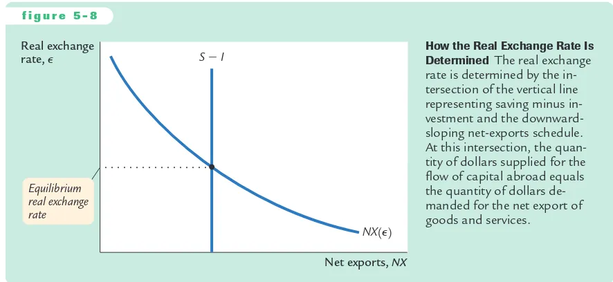
We now have all the pieces needed to construct a model that explains what fac-tors determine the real exchange rate. In particular, we combine the relationship between net exports and the real exchange rate we just discussed with the model of the trade balance we developed earlier in the chapter.We can summarize the analysis as follows:
➤ The real exchange rate is related to net exports.When the real exchange rate is lower, domestic goods are less expensive relative to foreign goods, and net exports are greater.
➤ The trade balance (net exports) must equal the net capital outflow, which in turn equals saving minus investment. Saving is fixed by the consump-tion funcconsump-tion and fiscal policy; investment is fixed by the investment func-tion and the world interest rate.
Figure 5-8 illustrates these two conditions.The line showing the relationship be-tween net exports and the real exchange rate slopes downward because a low real exchange rate makes domestic goods relatively inexpensive.The line representing the excess of saving over investment,S−I, is vertical because neither saving nor investment depends on the real exchange rate.The crossing of these two lines de-termines the equilibrium exchange rate.
Figure 5-8 looks like an ordinary supply-and-demand diagram. In fact, you can think of this diagram as representing the supply and demand for foreign-currency exchange.The vertical line,S−I, represents the net capital outflow and
thus the supply of dollars to be exchanged into foreign currency and invested abroad. The downward-sloping line,NX, represents the net demand for dollars coming from foreigners who want dollars to buy our goods.At the equilibrium real exchange rate, the supply of dollars available from the net capital outflow balances the de-mand for dollars by foreigners buying our net exports.
f i g u r e 5 - 8
Real exchange rate, e
Net exports, NX Equilibrium
real exchange rate
S 2 I
NX(e)
How the Real Exchange Rate Is Determined The real exchange rate is determined by the in-tersection of the vertical line representing saving minus in-vestment and the downward-sloping net-exports schedule. At this intersection, the quan-tity of dollars supplied for the
How Policies Influence the Real Exchange Rate
We can use this model to show how the changes in economic policy we dis-cussed earlier affect the real exchange rate.
Fiscal Policy at Home What happens to the real exchange rate if the
govern-ment reduces national saving by increasing governgovern-ment purchases or cutting taxes? As we discussed earlier, this reduction in saving lowers S−Iand thus NX.
That is, the reduction in saving causes a trade deficit.
Figure 5-9 shows how the equilibrium real exchange rate adjusts to ensure that NXfalls.The change in policy shifts the vertical S−Iline to the left,
low-ering the supply of dollars to be invested abroad. The lower supply causes the equilibrium real exchange rate to rise from
e
1toe
2—that is, the dollar becomesmore valuable. Because of the rise in the value of the dollar, domestic goods be-come more expensive relative to foreign goods, which causes exports to fall and imports to rise.The change in exports and the change in imports both act to re-duce net exports.
f i g u r e 5 - 9
Real exchange rate, e
Net exports, NX 1. A reduction in saving reduces the supply of dollars, . . .
2. . . . which raises the real exchange rate . . .
e 2
e 1
NX2 NX1
NX(e) S22 I S
12 I
3. . . . and causes net exports to fall.
The Impact of Expansionary Fiscal Policy at Home on the Real Exchange Rate Expansionary fi s-cal policy at home, such as an in-crease in government purchases or a cut in taxes, reduces na-tional saving. The fall in saving reduces the supply of dollars to be exchanged into foreign cur-rency, from S1−Ito S2−I. This shift raises the equilibrium real exchange rate from
e
1toe
2.Fiscal Policy Abroad What happens to the real exchange rate if foreign
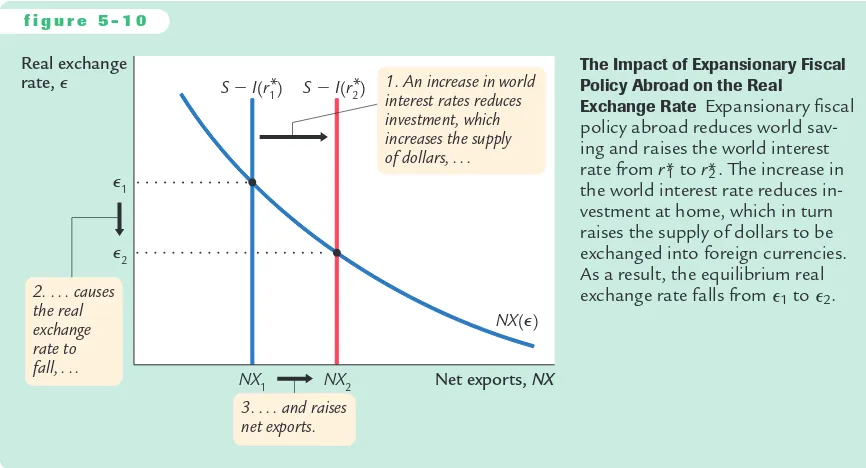
gov-ernments increase government purchases or cut taxes? This change in fiscal pol-icy reduces world saving and raises the world interest rate. The increase in the world interest rate reduces domestic investment I, which raises S − I and thus NX.That is, the increase in the world interest rate causes a trade surplus.
Figure 5-10 shows that this change in policy shifts the vertical S−Iline to the
User JOEWA:Job EFF01460:6264_ch05:Pg 133:26258#/eps at 100%
*26258*
Wed, Feb 13, 2002 9:27 AMShifts in Investment Demand What happens to the real exchange rate if invest-ment demand at home increases, perhaps because Congress passes an investinvest-ment tax credit? At the given world interest rate, the increase in investment demand leads to higher investment.A higher value of Imeans lower values of S−Iand NX.That is, the increase in investment demand causes a trade deficit.
Figure 5-11 shows that the increase in investment demand shifts the vertical S − I line to the left, reducing the supply of dollars to be invested abroad. The
f i g u r e 5 - 1 0
Real exchange rate, e
Net exports, NX
* *
1. An increase in world interest rates reduces investment, which increases the supply of dollars, . . .
The Impact of Expansionary Fiscal Policy Abroad on the Real
Exchange Rate Expansionary fiscal policy abroad reduces world sav-ing and raises the world interest rate from r* to 1 r*. The increase in2 the world interest rate reduces in-vestment at home, which in turn raises the supply of dollars to be exchanged into foreign currencies. As a result, the equilibrium real exchange rate falls from
e
1toe
2.f i g u r e 5 - 1 1
Real exchange rate, e
Net exports, NX e
The Impact of an Increase in Investment Demand on the Real Exchange Rate An increase in investment demand raises the quantity of domestic investment from I1to I2. As a result, the supply of dollars to be ex-changed into foreign currencies falls from S−I1to S−I2. This
fall in supply raises the equilib-rium real exchange rate from
e
1 toequilibrium real exchange rate rises. Hence, when the investment tax credit makes investing in the United States more attractive, it also increases the value of the U.S. dollars necessary to make these investments.When the dollar appreciates, domestic goods become more expensive relative to foreign goods, and net exports fall.
The Effects of Trade Policies
Now that we have a model that explains the trade balance and the real exchange rate, we have the tools to examine the macroeconomic effects of trade policies. Trade policies, broadly defined, are policies designed to influence directly the amount of goods and services exported or imported. Most often, trade policies take the form of protecting domestic industries from foreign competition— either by placing a tax on foreign imports (a tariff) or restricting the amount of goods and services that can be imported (a quota).
As an example of a protectionist trade policy, consider what would happen if the government prohibited the import of foreign cars. For any given real ex-change rate, imports would now be lower, implying that net exports (exports minus imports) would be higher.Thus, the net-exports schedule shifts outward, as in Figure 5-12. To see the effects of the policy, we compare the old equilib-rium and the new equilibequilib-rium. In the new equilibequilib-rium, the real exchange rate is higher, and net exports are unchanged. Despite the shift in the net-exports schedule, the equilibrium level of net exports remains the same, because the pro-tectionist policy does not alter either saving or investment.
f i g u r e 5 - 1 2
Real exchange rate, e
Net exports, NX e
1
e
2
S2 I
NX(e)
2
NX(e)
1
NX1 5 NX2
3. . . . but leave net exports unchanged. 2. . . . and
raise the exchange rate . . .
1. Protectionist policies raise the demand for net exports . . .
The Impact of Protectionist Trade Policies on the Real Exchange Rate A protectionist trade pol-icy, such as a ban on imported cars, shifts the net-exports schedule from NX(
e
)1to NX(e
)2, which raises the real exchange rate frome
1toUser JOEWA:Job EFF01460:6264_ch05:Pg 135:26260#/eps at 100%
*26260*
Wed, Feb 13, 2002 9:27 AM This analysis shows that protectionist trade policies do not affect the tradebalance. This surprising conclusion is often overlooked in the popular debate over trade policies. Because a trade deficit reflects an excess of imports over ex-ports, one might guess that reducing imports—such as by prohibiting the im-port of foreign cars—would reduce a trade deficit. Yet our model shows that protectionist policies lead only to an appreciation of the real exchange rate. The increase in the price of domestic goods relative to foreign goods tends to lower net exports by stimulating imports and depressing exports.Thus, the ap-preciation offsets the increase in net exports that is directly attributable to the trade restriction.
Although protectionist trade policies do not alter the trade balance, they do affect the amount of trade. As we have seen, because the real exchange rate ap-preciates, the goods and services we produce become more expensive relative to foreign goods and services.We therefore export less in the new equilibrium. Because net exports are unchanged, we must import less as well. (The appreci-ation of the exchange rate does stimulate imports to some extent, but this only partly offsets the decrease in imports caused by the trade restriction.) Thus, protectionist policies reduce both the quantity of imports and the quantity of exports.
This fall in the total amount of trade is the reason economists almost al-ways oppose protectionist policies. International trade benefits all countries by allowing each country to specialize in what it produces best and by providing each country with a greater variety of goods and services. Protectionist poli-cies diminish these gains from trade. Although these polipoli-cies benefit certain groups within society—for example, a ban on imported cars helps domestic car producers—society on average is worse off when policies reduce the amount of international trade.
The Determinants of the Nominal Exchange Rate
Having seen what determines the real exchange rate, we now turn our atten-tion to the nominal exchange rate—the rate at which the currencies of two countries trade. Recall the relationship between the real and the nominal ex-change rate:
Real Nominal Ratio of Exchange=Exchange× Price
Rate Rate Levels
e
= e × (P/P*). We can write the nominal exchange rate ase=
e
×(P*/P).exchange rate, if the domestic price level Prises, then the nominal exchange rate
ewill fall: because a dollar is worth less, a dollar will buy fewer yen. However, if the Japanese price level P* rises, then the nominal exchange rate will increase: because the yen is worth less, a dollar will buy more yen.
It is instructive to consider changes in exchange rates over time.The exchange rate equation can be written
% Change in e=% Change in
e
+% Change in P*−% Change in P.The percentage change in
e
is the change in the real exchange rate.Thepercent-age change in Pis the domestic inflation rate
p
, and the percentage change in P*is the foreign country’s inflation rate
p
*. Thus, the percentage change in thenominal exchange rate is
% Change in e=% Change in
e
+(p
*−p
)= +
This equation states that the percentage change in the nominal exchange rate between the currencies of two countries equals the percentage change in the real exchange rate plus the difference in their inflation rates.If a country has a high rate of inflation relative to the United States, a dollar will buy an increasing amount of the for-eign currency over time. If a country has a low rate of inflation relative to the United States, a dollar will buy a decreasing amount of the foreign currency over time.
This analysis shows how monetary policy affects the nominal exchange rate. We know from Chapter 4 that high growth in the money supply leads to high inflation. Here, we have just seen that one consequence of high inflation is a de-preciating currency: high
p
implies falling e. In other words, just as growth in theamount of money raises the price of goods measured in terms of money, it also tends to raise the price of foreign currencies measured in terms of the domestic currency.
Difference in Inflation Rates. Percentage Change in
Real Exchange Rate Percentage Change in
Nominal Exchange Rate
C A S E S T U D Y
Inflation and Nominal Exchange Rates
If we look at data on exchange rates and price levels of different countries, we quickly see the importance of inflation for explaining changes in the nominal exchange rate.The most dramatic examples come from periods of very high
in-flation. For example, the price level in Mexico rose by 2,300 percent from 1983 to 1988. Because of this inflation, the number of pesos a person could buy with a U.S. dollar rose from 144 in 1983 to 2,281 in 1988.
User JOEWA:Job EFF01460:6264_ch05:Pg 137:26262#/eps at 100%
*26262*
Wed, Feb 13, 2002 9:27 AM States (p
* −p
). On the vertical axis is the average percentage change in the ex-change rate between each country’s currency and the U.S. dollar (% change in e). The positive relationship between these two variables is clear in this figure. Countries with relatively high inflation tend to have depreciating currencies (you can buy more of them for your dollars over time), and countries with relatively low inflation tend to have appreciating currencies (you can buy less of them for your dollars over time).As an example, consider the exchange rate between German marks and U.S. dollars. Both Germany and the United States have experienced inflation over the past twenty years, so both the mark and the dollar buy fewer goods than they once did. But, as Figure 5-13 shows, inflation in Germany has been lower than inflation in the United States. This means that the value of the mark has fallen less than the value of the dollar.Therefore, the number of German marks you can buy with a U.S. dollar has been falling over time.
f i g u r e 5 - 1 3
Percentage change in nominal exchange rate
10 9 8 7 6 5 4 3 2 1 0 21 22 23 24
Inflation differential
Depreciation relative to U.S. dollar
Appreciation relative to U.S. dollar
21 22
23 0 1 2 3 4 5 6 7 8
France Canada
Sweden Australia
UK Ireland
Spain
South Africa
Italy
New Zealand
Netherlands Germany
Japan Belgium
Switzerland
Inflation Differentials and the Exchange Rate This scatterplot shows the relationship between inflation and the nominal exchange rate. The hori-zontal axis shows the country’s average inflation rate minus the U.S. aver-age inflation rate over the period 1972–2000. The vertical axis is the average percentage change in the country’s exchange rate (per U.S. dollar) over that period. This figure shows that countries with relatively high infl a-tion tend to have depreciating currencies and that countries with relatively low inflation tend to have appreciating currencies.
The Special Case of Purchasing-Power Parity
A famous hypothesis in economics, called the law of one price, states that the same good cannot sell for different prices in different locations at the same time. If a bushel of wheat sold for less in New York than in Chicago, it would be prof-itable to buy wheat in New York and then sell it in Chicago. Astute arbitrageurs would take advantage of such an opportunity and, thereby, would increase the demand for wheat in New York and increase the supply in Chicago.This would drive the price up in New York and down in Chicago—thereby ensuring that prices are equalized in the two markets.
The law of one price applied to the international marketplace is called purchasing-power parity. It states that if international arbitrage is possible, then a dollar (or any other currency) must have the same purchasing power in every country. The argument goes as follows. If a dollar could buy more wheat domestically than abroad, there would be opportunities to profit by buying wheat domestically and selling it abroad. Profit-seeking arbitrageurs would drive up the domestic price of wheat relative to the foreign price. Similarly, if a dollar could buy more wheat abroad than domestically, the arbitrageurs would buy wheat abroad and sell it domestically, driving down the domestic price relative to the foreign price.Thus, profit-seeking by international arbitrageurs causes wheat prices to be the same in all countries.
We can interpret the doctrine of purchasing-power parity using our model of the real exchange rate. The quick action of these international arbitrageurs im-plies that net exports are highly sensitive to small movements in the real ex-change rate. A small decrease in the price of domestic goods relative to foreign goods—that is, a small decrease in the real exchange rate—causes arbitrageurs to buy goods domestically and sell them abroad. Similarly, a small increase in the relative price of domestic goods causes arbitrageurs to import goods from abroad. Therefore, as in Figure 5-14, the net-exports schedule is very flat at the real exchange rate that equalizes purchasing power among countries: any small
f i g u r e 5 - 1 4
Real exchange rate, e
Net exports, NX
NX(e) S2 I
User JOEWA:Job EFF01460:6264_ch05:Pg 139:26264#/eps at 100%
*26264*
Wed, Feb 13, 2002 9:27 AM movement in the real exchange rate leads to a large change in net exports.Thisextreme sensitivity of net exports guarantees that the equilibrium real exchange rate is always close to the level ensuring purchasing-power parity.
Purchasing-power parity has two important implications. First, because the net-exports schedule is flat, changes in saving or investment do not influence the real or nominal exchange rate. Second, because the real exchange rate is fixed, all changes in the nominal exchange rate result from changes in price levels.
Is this doctrine of purchasing-power parity realistic? Most economists believe that, despite its appealing logic, purchasing-power parity does not provide a completely accurate description of the world. First, many goods are not easily traded. A haircut can be more expensive in Tokyo than in New York, yet there is no room for international arbitrage because it is impossible to transport haircuts. Second, even tradable goods are not always perfect substitutes. Some consumers prefer Toyotas, and others prefer Fords. Thus, the relative price of Toyotas and Fords can vary to some extent without leaving any profit opportunities. For these reasons, real exchange rates do in fact vary over time.
Although the doctrine of purchasing-power parity does not describe the world perfectly, it does provide a reason why movement in the real exchange rate will be limited.There is much validity to its underlying logic: the farther the real exchange rate drifts from the level predicted by purchasing-power parity, the greater the incentive for individuals to engage in international arbitrage in goods. Although we cannot rely on purchasing-power parity to eliminate all changes in the real exchange rate, this doctrine does provide a reason to expect that fluctuations in the real exchange rate will typically be small or temporary.1
1To learn more about purchasing-power parity, see Kenneth A. Froot and Kenneth Rogoff,“
Per-spectives on PPP and Long-Run Real Exchange Rates,”in Gene M. Grossman and Kenneth Ro-goff, eds.,Handbook of International Economics, vol. 3 (Amsterdam: North-Holland, 1995).
C A S E S T U D Y
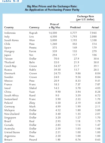
The Big Mac Around the World
The doctrine of purchasing-power parity says that after we adjust for exchange rates, we should find that goods sell for the same price everywhere. Conversely, it says that the exchange rate between two currencies should depend on the price levels in the two countries.
To see how well this doctrine works, The Economist, an international news-magazine, regularly collects data on the price of a good sold in many countries: the McDonald’s Big Mac hamburger. According to purchasing-power parity, the price of a Big Mac should be closely related to the country’s nominal exchange rate.The higher the price of a Big Mac in the local currency, the higher the ex-change rate (measured in units of local currency per U.S. dollar) should be.
cost 294 yen in Japan, we would predict that the exchange rate between the dollar and the yen was 294/2.51, or 117, yen per dollar.At this exchange rate, a Big Mac would have cost the same in Japan and the United States.
Table 5-2 shows the predicted and actual exchange rates for 30 countries, ranked by the predicted exchange rate. You can see that the evidence on purchasing-power
Exchange Rate (per U.S. dollar) Price of
Country Currency a Big Mac Predicted Actual
Indonesia Rupiah 14,500 5,777 7,945
Italy Lira 4,500 1,793 2,088
South Korea Won 3,000 1,195 1,108
Chile Peso 1,260 502 514
Spain Peseta 375 149 179
Hungary Forint 339 135 279
Japan Yen 294 117 106
Taiwan Dollar 70.0 27.9 30.6
Thailand Baht 55.0 21.9 38.0
Czech Rep. Crown 54.37 21.7 39.1
Russia Ruble 39.50 15.7 28.5
Denmark Crown 24.75 9.86 8.04
Sweden Crown 24.0 9.56 8.84
Mexico Peso 20.9 8.33 9.41
France Franc 18.5 7.37 7.07
Israel Shekel 14.5 5.78 4.05
China Yuan 9.90 3.94 8.28
South Africa Rand 9.0 3.59 6.72
Switzerland Franc 5.90 2.35 1.70
Poland Zloty 5.50 2.19 4.30
Germany Mark 4.99 1.99 2.11
Malaysia Dollar 4.52 1.80 3.80
New Zealand Dollar 3.40 1.35 2.01
Singapore Dollar 3.20 1.27 1.70
Brazil Real 2.95 1.18 1.79
Canada Dollar 2.85 1.14 1.47
Australia Dollar 2.59 1.03 1.68
United States Dollar 2.51 1.00 1.00
Argentina Peso 2.50 1.00 1.00
Britain Pound 1.90 0.76 0.63
Note: The predicted exchange rate is the exchange rate that would make the price of a Big Mac
in that country equal to its price in the United States. Source: The Economist, April 29, 2000, 75.
User JOEWA:Job EFF01460:6264_ch05:Pg 141:26266#/eps at 100%
*26266*
Wed, Feb 13, 2002 9:27 AM5-4
Conclusion: The United States as a Large
Open Economy
In this chapter we have seen how a small open economy works.We have exam-ined the determinants of the international flow of funds for capital accumulation and the international flow of goods and services.We have also examined the de-terminants of a country’s real and nominal exchange rates. Our analysis shows how various policies—monetary policies,fiscal policies, and trade policies—affect the trade balance and the exchange rate.
The economy we have studied is “small’’in the sense that its interest rate is fixed by world financial markets. That is, we have assumed that this economy does not affect the world interest rate, and that the economy can borrow and lend at the world interest rate in unlimited amounts. This assumption contrasts with the assumption we made when we studied the closed economy in Chapter 3. In the closed economy, the domestic interest rate equilibrates domestic saving and domestic investment, implying that policies that influence saving or invest-ment alter the equilibrium interest rate.
Which of these analyses should we apply to an economy such as the United States? The answer is a little of both. The United States is neither so large nor so isolated that it is immune to developments occurring abroad.The large trade deficits of the 1980s and 1990s show the importance of international financial markets for funding U.S. investment. Hence, the closed-economy analysis of Chapter 3 cannot by itself fully explain the impact of policies on the U.S. economy.
Yet the U.S. economy is not so small and so open that the analysis of this chapter applies perfectly either. First, the United States is large enough that it can influence world financial markets. For example, large U.S. budget deficits were often blamed for the high real interest rates that prevailed throughout the world in the 1980s. Second, capital may not be perfectly mobile across countries. If in-dividuals prefer holding their wealth in domestic rather than foreign assets, funds for capital accumulation will not flow freely to equate interest rates in all coun-tries. For these two reasons, we cannot directly apply our model of the small open economy to the United States.
When analyzing policy for a country such as the United States, we need to combine the closed-economy logic of Chapter 3 and the small-open-economy logic of this chapter.The appendix to this chapter builds a model of an economy between these two extremes. In this intermediate case, there is international bor-rowing and lending, but the interest rate is not fixed by world financial markets. Instead, the more the economy borrows from abroad, the higher the interest rate it must offer foreign investors. The results, not surprisingly, are a mixture of the two polar cases we have already examined.
Consider, for example, a reduction in national saving caused by a fiscal expan-sion. As in the closed economy, this policy raises the real interest rate and crowds out domestic investment. As in the small open economy, it also reduces the net capital outflow, leading to a trade deficit and an appreciation of the exchange rate. Hence, although the model of the small open economy examined here does not precisely describe an economy such as the United States, it does provide ap-proximately the right answer to how policies affect the trade balance and the ex-change rate.
Summary
1.Net exports are the difference between exports and imports. They are equal to the difference between what we produce and what we demand for con-sumption, investment, and government purchases.
2.The net capital outflow is the excess of domestic saving over domestic invest-ment.The trade balance is the amount received for our net exports of goods and services.The national income accounts identity shows that the net capital outflow always equals the trade balance.
3.The impact of any policy on the trade balance can be determined by examing its impact on savexaming and investment. Policies that raise savexaming or lower in-vestment lead to a trade surplus, and policies that lower saving or raise investment lead to a trade deficit.
4.The nominal exchange rate is the rate at which people trade the currency of one country for the currency of another country. The real exchange rate is the rate at which people trade the goods produced by the two countries.The real exchange rate equals the nominal exchange rate multiplied by the ratio of the price levels in the two countries.
5.Because the real exchange rate is the price of domestic goods relative to for-eign goods, an appreciation of the real exchange rate tends to reduce net ex-ports.The equilibrium real exchange rate is the rate at which the quantity of net exports demanded equals the net capital outflow.