COMPARISON OF SPOT AND LANDSAT DATA IN CLASSIFYING WETLAND
VEGETATION TYPES
Matsie T. Mosime1 and Solomon G. Tesfamichael1
1Department of Geography, Environmental Management and Energy Studies, University of Johannesburg, PO Box 524,
Auckland Park 2006, South Africa
Email: [email protected] and [email protected]
KEY WORDS: Wetland vegetation, SPOT, Landsat, Unsupervised classification, Klipriviersberg Nature Reserve
ABSTRACT:
The aim of this study was to compare the performances of Landsat and SPOT imagery to map wetland vegetation types in the Klipsriviersberg Nature Reserve, South Africa. The Gauteng Conservation Plan 3.3 (C-Plan 3) was used to delineate the boundaries of the wetlands in the study area. According to the plan, the proposed study area falls within the Critical Biodiversity Areas (CBA) and Ecological Support Areas (ESA). Limited field data were collected within the boundaries of the wetlands during summer 2015 when the vegetation cover was relatively high. These data identified features including sparse vegetation, dense vegetation, grassland and bare land.Additional samples were added from Google Earth image to increase sample size. Both the field data and Google Earth data were used as reference against which the performances of SPOT and Landsat product were compared. Unsupervised classification was used to classify SPOT and Landsat images acquired in summer 2015. The results showed that overall accuracy of SPOT images is higher than Landsat images. This is attributed to its high spatial resolution of 1.5 m compared to 30 m spatial resolution of Landsat imagery. This indicates that SPOT imagery is recommended to map wetland vegetation diversity in a localised area such as the study area. The current high temporal resolution of the image has also an added advantage that conservationists should exploit.
1. INTRODUCTION
Wetlands are important resources which play many functional purposes in an ecosystem. They share a common feature of retaining excess water, long enough to influence land uses, soil characteristics and life forms (Fuggie & Rubbie, 2009). Wetlands are therefore considered to be one of the richest biomes that support biological diversity and ecological services. They are home to large numbers of terrestrial, amphibious organisms and birds. Due to their importance to both the environment and human beings, wetlands are subjected to enormous pressure from both human activities (Bassi, 2016).
The importance of wetlands and their management has gained increasing recognition in many parts of the world (Islam et al., 2008). Thus, a reliable inventory and map of wetland systems is very useful to understand the spatial distribution of different wetlands and their linkage with other land units. This will help in planning, management and conservation of wetlands (Islam et al., 2008; Rebelo & Nagabhatla, 2009). Remote sensing offers the opportunity to map and inventory wetlands rapidly and consistently, irrespective of the geographic location (Islam et al., 2008). The approach covers large areas, and is cost- and time efficient making it for wetland characterization (Xie et al., 2008). Due to lack of efficient monitoring techniques of wetland vegetation types, the level of success in protecting wetlands is limited (Dutcher, 2013). In Klipsriviersberg Nature Reserve, several vegetation surveys have been conducted in the last few decades but none produced a practical, useable map for environmental management purposes. Therefore, a suitable methodology to map vegetation diversity in the wetlands of the reserve is to enable efficient management (KNRA, 2015). Remote sensing provides useful techniques in characterizing wetland ecosystems. Kayastha et al. (2013) used inter-annual time series of Landsat data from 1985 to 2009 to map changes in wetland ecosystems development, harvesting, thinning and farming practices in northern Virginia. The study reported the
utility of the approach within acceptable degrees of confidence. Similarly, Sghair & Goma (2013) used Landsat data, aerial photographs and field observations to assess wetland vegetation change over time at two contrasting wetland sites (freshwater wetland and salt marsh) in the UK. The results showed a substantial temporal change in vegetation for the former and a slight change in the latter wetland type. The study concluded that remote sensing could provide useful baseline data about wetland vegetation change over time and across expansive areas, which can be instrumental in the management and conservation of wetland habitats. Fickas et al. (2016) used Landsat data from 1972 to 2012 to evaluate wetland change in Willamette River of
Oregon’s Willamette Valley. The study showed that the wetland experienced annual losses and gains due to urbanisation and agricultural activities. Such studies have demonstrated the performances of remote sensing in characterizing large wetland environments. There is a need to apply the technology in smaller wetland systems. In this regard, it is important to determine the effect of spatial resolution on identifying vegetation types within a relatively small wetland area. The main of this study was therefore to compare the performance of Landsat and SPOT imagery to map wetland vegetation types in the Klipsriviersberg Nature Reserve, South Africa.
2. METHODS
2.1 Study area
with approximately 650 indigenous plant species, 215 bird species, 16 reptile species and 32 butterfly species.
Figure 1: Klipsriviersberg Nature Reserve
2.2 Reference data
Field data and Google Earth™ image were used as reference data.
Field data were collected within the boundaries of the Gauteng Conservation Plan 3.3, that identifies sites that are critical for maintaining biodiversity, during summer season when the vegetation cover is relatively high. Thirty sample points were laid within the wetland boundaries using a random sampling technique. The geographic coordinates of these points were recorded using GPS (Global Positioning System) at 3 m accuracy. A circular plot with a radius of 30 m was placed around each point and within the wetland boundary for sampling purpose. A line transect was laid between the centre and the periphery of the plot in the north, south, east and west directions. Features such as trees, bush, plants, rocks and grass were recorded at 10 m interval along each transect line. Due to limited data and time, field surveys were not sufficient; therefore, 40 more samples were increased by interpreting similar features on
Google Earth™ image acquired during the time of the field survey. The Google Earth™ image has high spatial resolution
(0.5 m) and can be used as a source of reference data (Potere, 2008; Jaafari & Nazarisamani, 2013). The Google Earth™ image was acquired in May 2015 and was obtained from Google Earth Pro. The combination of field survey and Google Earth based sampling resulted in a total of 70 samples.
2.3 Remotely-sensed data
One of the objectives of the study was to compare the performance of SPOT 7 and Landsat imagery, both of which were acquired in May 2015 to map wetland vegetation types in the reserve. SPOT 7 image, which was obtained from South African National Space Agency, had a spatial resolution of 1.5 m and a temporal resolution of a day (Ozesmi & Bauer, 2002). SPOT imagery has been found useful for studying, monitoring, forecasting and managing natural resources and human activities (Xie et al., 2008). Landsat image were downloaded from the
United States Geological Survey’s online portal
(http://earthexplorer.usgs.gov/). The Landsat image was already geometrically corrected (Level 1). Landsat images have a 30 m spatial resolution and a temporal resolution of 16 days. The spectral resolution of Landsat imagery makes it suitable to identify vegetation types, health conditions and measure reflectance peak of green vegetation (Klemas, 2011). The
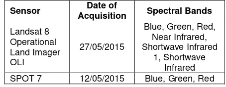
characteristics of the imagery used in this study are presented in Table 1.
Sensor Acquisition Date of Spectral Bands
Landsat 8
Table 1: Characteristics of data used in the study
2.4 Data analysis
2.4.1 Image processing
Both SPOT and Landsat images were made available terrain corrected and hence it was unnecessary to apply geometric correction. Cloud free images were used to avoid the effects of clouds and their shadows on the ground. As a result, atmospheric correction was not applied on the images. The images were classified to produce thematic maps. Image classification is the grouping of pixels into different land cover types based on spectral values (Lillesand, 2008). Unsupervised classification and ISODATA (Iterative Self Organizing Data Analysis) algorithm available in ArcGIS software (ESRI® ArcGIS version 10.3, Redlands, CA) was used for the classification. Unsupervised classification was used because it does not require prior knowledge; instead it uses statistical information to assign pixels to spectrally distinct classes (Campbell & Wynne, 2011). The ISODATA algorithm uses an iterative process in which the user defined number of clusters, k, are assigned arbitrary cluster means in multidimensional attribute space. All of the data points are then assigned to these clusters and new means are recalculated for every class. Using these new means, the data are then reclassified to the nearest cluster in attribute space and the cluster means are recalculated (Karila et al., 2014). This process is repeated until a specified maximum number of iterations have been performed, or a maximum percentage of unchanged pixels have been reached between two successive iterations for a specified number of classes (Sghair & Goma, 2013).
The images were classified into four land cover classes: (1) dense vegetation (2) sparse vegetation (3) grass land and (4) bare land. Grassland is defined as an area covered by grass species especially for grazing, forbs and few or no trees and shrubs (Simpson & Weiner, 1989; Schimdt et al., 2002; Kafi et al., 2014). Sparse vegetation describes an area of land where plant growth may be scattered or disperse (Trisakti, 2017). Yuvaraj et al. (2014) defines dense vegetation as an area consisting of stunted trees or bushes. Bare land is described as exposed soils, landfill sites and areas of active excavation (Dewan & Yamaguchi, 2009). The classes were interpreted by using different band combinations such as including red-green-blue (RGB) and (near-infrared-red-green) colour composites.
2.4.2 Accuracy assessment
vegetation types in the reserve. The assessment was performed by comparing classes derived from SPOT and Landsat with the
reference data obtained from Google Earth™ image. An error or
confusion matrix was used to assess accuracies of the SPOT and Landsat map. An error matrix is a square array of numbers set out in rows and columns which express the number of sample units assigned to a particular class relative to the actual class on the reference data (Congalton & Green, 2009). The assessment uses
various statistical tools such as overall, producer’s and user’s
accuracies as well as Kappa (K-hat) coefficient to determine accuracy levels. Overall accuracy is the total classification accuracy, and is obtained by dividing the total number of correct pixels of all classes by the total number of pixels in the sample.
Producer’s accuracy is a measure of how well a certain area is
classified, and is calculated by dividing the number of correctly classified points for each class by the number of reference points of that category (Congalton & Green, 2009). The user's accuracy is a measure of the reliability of the classification or the probability that a pixel on a map actually represents that class on the ground. It is calculated by dividing the number of pixels correctly classified by the total number of pixels categorized in that class (Congalton, 1991). Kappa coefficient is a measure used to determine whether the results in the error matrix are significantly better than a random result (K-hat = 0) (Congalton, 1991). K-hat is computed using Equation 1 (Congalton, 1991): � = 1− ℎ �− ℎ� � ...Equation 1
3. RESULTS AND DISCUSSIONS
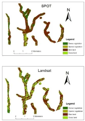
Figure 2 shows the final maps derived from the two images. The figure demonstrates that bare land cover is more dominant in SPOT image than in Landsat image. Further, the figure shows that SPOT image is visually smoother compared to Landsat derived classes. The overall accuracy and kappa coefficient is higher for SPOT image (Table 2) than for Landsat (Table 3). The high SPOT overall accuracy and kappa coefficient are attributed to its spatial resolution of 1.5 m. According to the guidelines of Landis and Kosh (1977) and Fleiss (1981), the kappa coefficient obtained for SPOT and Landsat can be considered moderate and fair, respectively. Furthermore, SPOT data illustrates that the producer accuracies for dense vegetation and grassland is 62% and 60% respectively, whereas, user’s accuracies for dense vegetation and grassland is 77% and 75% respectively. Moreover, SPOT data illustrates that the producer accuracies for bare land and sparse vegetation is 80% and 77% respectively, whereas, the user accuracies for bare land and sparse vegetation in SPOT data is 76% and 66% respectively. These results indicate that the classification using SPOT did well to detect dense vegetation, grassland, bare land and sparse vegetation. In
contrast, the producer’s accuracies for bare land, dense vegetation, sparse vegetation and grass land were 44%, 82%,
60% and 47% respectively; while the corresponding user’s
accuracies were 60%, 81%, 40% and 38%, showing the inferiority of classification using Landsat data.
The findings of this study are consistent with the study by Huili et al. (2011) who revealed that SPOT data (2.5 m) had a better overall accuracy than Landsat (30 m). Na et al. (2015) used Landsat to map wetlands in the Great Zhan River Basin and reported a better overall accuracy of 85.97%. However, their study included additional data namely synthetic aperture radar (SAR) and topographical indices.
Figure 2: SPOT and Landsat derived classes
REFERENCE
Table 2: SPOT accuracy assessment (BL=Bare land; DV=Dense vegetation; SV=Sparse vegetation; GL=Grass land)
REFERENCE
4. CONCLUSION
The study revealed that SPOT had a better performance compared to Landsat. This is attributed to its high spatial resolution of 1.5 m compared to 30 m spatial resolution of Landsat imagery. SPOT imagery is therefore recommended to map wetland vegetation in localised areas such as the study area. Although, Landsat data can still be used as an option since it has a better spectral resolution; however methods such as spectral pan-sharpening to improve its spatial performance.
5. ACKNOWLEDGEMENTS
We would like to thank the University of Johannesburg for partly funding this project. We would also like thank the International Symposium on Remote Sensing of Environment (ISRSE) for funding participation at the ISRSE37 conference.
6. REFERENCE
Bassi, N. 2016: Implications of institutional vacuum in wetland conservation for water management. IIM Kozhikode Society & Management Review, 5(1), pp. 41-50.
Campbell, B.J. & Wynne, R.H. 2011: Introduction to Remote Sensing, (5th Ed.), New York: Guilford.
Congalton, R.G. 1991: A review of assessing the accuracy of classifications of remotely sensed Data. Remote Sensing of Environment, 37(1), pp. 35-46.
Congalton, R.G. & Green, K. 2009: Assessing the accuracy of remotely sensed data, principles and practice (2nd Ed.) New
York: Tylor & Francis Group.
Dinar, A. Hassan, R. Mendelsohn, R. & Benhin, J. 2012: Climate change and agriculture in Africa: impact assessment and adaptation strategies. Routledge: Taylor & Francis.
Dutcher, N. 2013: Towards a characterization of wetland invasive vegetation using a combination of field and remote sensing techniques. Unpublished MSc thesis. Rochester Institute of Technology. New York.
Dewan, A.M. & Yamaguchi, Y. 2009: Using remote sensing and GIS to detect and monitor land use and land cover change in Dhaka Metropolitan of Bangladesh during 1960-2005, Environmental Monitoring and Assessment, 150, pp. 237-249. Fuggle, R.F. & Rabie, M.A. 2005: Environmental management in South Africa. Cape Town: Juta & Co Ltd.
Gauteng department of agriculture and rural development, 2014: Technical report for the Gauteng conservation plan http://www.gdard.gpg.gov.za/Publications1/AGRICULTURE% 20APP.pdf (08 May. 2016).
Islam, A. Thenkabail, P. S. Kulawardhana, R. W. Alankara, R. Gunasinghe, S. Edussriya, C. & Gunawardana, A. 2008: Semi‐ automated methods for mapping wetlands using Landsat ETM+ and SRTM data. International Journal of Remote Sensing, 29(24), pp. 7077-7106.
Jaafari, S. & Nazarisamani, A. 2008: Comparison between land use/land cover mapping through Landsat and Google Earth imagery. American-Eurasian Journal of Agricultural and Environmental Sciences, 13(6), pp.763-768.
Kafi, K.M. Shafri, H.Z.M.A. & Shariff, B.M. 2014: An analysis of LULC change detection using remotely sensed data; a case study of Bauchi City. IOP Conference Series: Earth and Environmental Science, 20, pp. 012-056.
Karila, K. Nevalainen, O. Krooks, A. Karjalainen, M & Kaasalainen, S. 2014: Monitoring changes in rice cultivated area from SAR and optical satellite images in Ben Tre and TraVinhprovinces in Mekong Delta, Vietnam. Remote Sensing, 6, pp. 4090-4108.
Klemas, V. 2011: Remote sensing of wetlands; case studies comparing practical techniques. Journal of Coastal Research, 27(3), pp. 418-427.
KNRA, 2015: Kliprievrsberg
http://www.klipriviersberg.org.za/index.php/geology (18 September. 2015).
Kayastha, N. 2013: Application of light detection and ranging (LiDAR) and multi-temporal Landsat for mapping and monitoring wetlands. Unpublished Phd thesis. Virginia Polytechnic Institute and State University. Blacksburg.
Fickas, K.C. Cohen, W.B. & Yang, Z. 2016: Landsat-based monitoring of annual wetland change in the Willamette Valley of Oregon, USA from 1972 to 2012. Wetlands Ecology Management, 24, 73-92.
Lillesand, T.M., Kiefer, R.W. & Chipman, J.W. 2008: Remote Sensing and Image Interpretation (6th Ed.), New York: John
Wiley & Sons Inc.
Mai, M. 2010: Groundwater study of a subtropical small-scale wetland GaMampa wetland, Mohlapetsi River catchment, Olifants River basin, South Africa) http://www.wetwin.eu/downloads/CS-SA-2.pdf(June 20. 2015).
Motswaledi, M. 2015: Using remote sensing indices to evaluate habitat intactness in the Bushbuckridge area, a key to effective planning. Unpublished Bsc Honours thesis. Stellenbosch University. South Africa.
Mthiyane, T.S. 2009: Small scale farming on wetland resource utilisation: a case study of Mandlanzini, Richards Bay http://uzspace.uzulu.ac.za/bitstream/handle/10530/550/small%2 0scale%20farming%20on%20wetlang%20resource.pdf?sequenc e=1(January 01. 2016).
Na, X. D. Zang, S. Y. Wu, C. S. & Li. W. L. 2015: Mapping forested wetlands in the Great Zhan River Basin through integrating optical, radar, and topographical data classification techniques. Environmental Monitoring Assessment, 187, 696, DOI 10.1007/s10661-015-4914-7.
Potere, D. 2008: Horizontal positional accuracy of Google
Earth’s high resolution. Imagery Archive Sensors, 8, pp. 7973-7981.
Rai, V. 2008: Modeling a wetland system-the case of Keoladeo National Park (KNP), India. Ecological Modelling, 210(3): 247-252.
Rebelo, L.M. Finlayson, C.M. & Nagabhatla, N. 2009: Remote sensing and GIS for wetland inventory, mapping and change analysis. Journal of Environmental Management, 90, pp. 2144-2153.
Schimdt, E. Lotter, M. & Mcclaland, W. 2002: Trees and shrub of Mpumalanga and Kruger National Park (1st Ed.), South
Africa. Jacana Media.
Simpson, J.A. & Weiner, E.S.C. 1989: The oxford english dictionary (2nd Ed.), volume vi, Oxford: Clarendon Press.
Sghair, A. & Goma, F. 2013: Remote sensing and GIS for wetland vegetation study. PhD thesis. Unpublished PhD thesis. University of Glasgow. Scotland.
Shi, Y. 2013: A remote sensing and GIS based wetland analysis in Canaan valley, West Virginia. Unpublished MSc thesis. Marshall University. United States of America.
Solaimani, K. Arekhi, M. Tamartash, R. & Miryaghobzadeh, M. 2010: Land use/cover change detection based on remote sensing data (A case study; Neka Basin) http://www.cabdirect.org/abstracts/20113247757.html;jsessioni d=B5105E4F8BF4675EF9DFC0978CE2F221?freeview=true (06 June. 2016).
Trisakti, B. 2017: Vegetation type classification and vegetation cover percentage estimation in urban green zone using pleiadesimagery. IOP Conference Series Earth and Environmental Science, 54, 012003 doi:10.1088/1755-1315/54/1/012003.
USGS, 2015: Landsat missions, United States Geological Survey http://earthexplorer.usgs.gov/(24 November. 2015).