94
NETWORKS: A SURVEY
Lanny Sitanayah
Dept. of Computer Science, University College Cork Cork, Ireland
E-mail: [email protected]
ABSTRACT: Wireless sensor networks (WSNs) comprise a large number of sensor nodes, which are spread out within a region and communicate using wireless links. In some WSN applications, recognizing boundary nodes is important for topology discovery, geographic routing and tracking. In this paper, we study the problem of recognizing the boundary nodes of a WSN. We firstly identify the factors that influence the design of algorithms for boundary detection. Then, we classify the existing work in boundary detection, which is vital for target tracking to detect when the targets enter or leave the sensor field.
Keywords: Wireless sensor networks, boundary detection, algorithms.
INTRODUCTION
Rapid improvements in wireless communication and electronics technologies have enabled the development of small, low-cost, low-power, multi-functional devices: sensor nodes. A sensor node (or mote) is a battery-powered device with integrated sensing, processing and communication capabilities. It can detect and monitor changes in a variety of physical conditions, such as temperature, humidity, light, sound, chemicals, or the presence of certain objects [1]. Nodes can perform simple computations and communicate with each other over short distances using radio.
A wireless sensor network (WSN) is composed of up to thousands of unattended sensor nodes and one or more base stations. The sensor nodes are deployed either densely or sparsely, manually or randomly, in a region to be monitored, for example, natural environments, battlefields, hospitals, houses and industries. Unlike the sensor nodes which have limited power, storage, processing and communica-tion capabilities, a base stacommunica-tion has more energy, storage, processing and communication resources. Base stations, such as laptops and other wireless hand-held devices, act as gateways between sensor nodes and an end-user. That is, the sensor readings are sent to the base station to be saved in a database and the end-user can retrieve and use this information as needed. Figure 1 illustrates a typical WSN confi-guration.
The arrangement and management of a WSN depends on the application for which it is used [2], such as:
1. Military applications: tracking enemy vehicles, detecting illegal border crossings and monitoring friendly troops.
2. Environmental applications: habitat monitoring, animal tracking (tracking of moving birds, small animals and insects), flood and forest fire detections. 3. Health applications: telemonitoring of human
physiological data, tracking and monitoring doctors and patients inside a hospital.
4. Home applications: home appliances automation. 5. Other commercial applications: vehicle tracking
and detection.
WSN applications are categorized into periodic and event detection data gathering. Periodic data gathering applications require sensor nodes to send their sensing data to the base station periodically. Habitat monitoring at Great Duck Island [3] is an example of a periodic data gathering application. In the event detection data gathering applications, sensor nodes send monitoring data to the base station only when an event of interest occurs in the sensor field. For example, forest fire detections [4, 5], building fire detections [6] and moving object tracking.
In many WSN applications that involve moving objects (or targets), the most important task of WSN is target tracking. WSNs for target tracking have three important operations: detecting, monitoring and reporting [7]. In the detection operation, sensor nodes must be able to detect the targets when they cross the monitoring area. Unfortunately, having all nodes to sense for incoming targets at all times is not energy efficient. Instead, only nodes which are located on the boundary of the network are set to be active and sense the targets. The process of finding boundary nodes is called boundary detection.
Once the boundary has been detected, during the monitoring period, sensor nodes have to track the targets until they leave the network. In this period, nodes may be able to predict the targets' movement and alert only nodes on the predicted track to continue tracking. Finally, in the reporting operation, sensor nodes that sense the targets have to report the detection and the movement of the targets to the applications. Nodes can also report the direction and the location of the targets if the information is available. Monitoring and reporting operations are interleaved during the entire target tracking process [8]. In this paper, we focus our study on the detecting and monitoring operations, specifically on boundary detection.
ALGORITHM DESIGN FOR BOUNDARY DETECTION boundary nodes is simplified if the exact location of each sensor node in the monitoring area is known. Unfortunately, building a large scale WSN with special location hardware such as GPS embedded in the nodes is not practical [9], because:
The price of GPS is expensive compared to the nodes themselves, so it is not cost effective. The considerable amount of nodes' energy that is consumed by GPS will lead to short lifetime networks, hence it is not energy efficient.
GPS cannot function well in a closed place where the microwave signal from the satellites is blocked by obstacles.
The size of GPS and its antenna can increase the size and change the structure of the nodes, but many applications require small sensor nodes.
For that reason, some measurement techniques to localize sensor nodes such as AOA (angle-of-arrival), TDOA (time-difference-of-arrival) and distance-based measurement exist [10]. In [10], Mao et al. focus the investigation on distance-based sensor network localization. They describe several distri-buted and centralized distance-based localization algorithms. These algorithms localize sensor nodes with regard to some landmarks or estimate relative sensor locations. Unfortunately, such localization techniques have several drawbacks. Firstly, the computational complexity of the algorithms is high. Secondly, for some applications that require a global coordinate system, the localization algorithms still need several sensor nodes with known location information (anchors) in order to localize other nodes without location information (non-anchors).
Centralized vs distributed algorithm
A centralized algorithm relies on one central node which is usually the base station to perform the whole computation based on the global information of the network. Instead, a distributed algorithm performs the computation task based on local information. In many WSN applications, sensor nodes are scattered randomly in the monitoring region. This random deployment does not guarantee that the whole network is connected. Furthermore, nodes may be broken or destroyed before they can perform their mission. This condition leads to partitions of the network and some partitions may be unreachable by multi-hop communication to the base station for centralized processing. Hence, distributed or decentralized algorithms are preferable to centralized algorithms in WSN applications.
Low density networks
Robustness
WSN algorithms must be robust to any uncertainties of the monitoring environment, such as inactive or malfunctioning nodes, broken communicate-on links, disccommunicate-onnected networks and any faulty measurements, such as erroneous distance measure-ments between nodes.
Accuracy
WSN algorithms that involve target detection and tracking must be accurate, so the targets are not lost during the monitoring period. Accuracy is usually measured by false alarms (or false positives) and misses (or false negatives) [12]. In target detection, a false positive happen when a target is incorrectly detected but in fact there are no targets in the network. Conversely, a false negative is when a target is not detected but in fact the target is present.
Energy efficiency
Energy efficiency is one of the most critical factors for WSN applications, especially target tracking. The application needs a lot of sensing, processing and communication to track a target accurately. The lower the energy consumed by each node, the longer the network can perform its mission. Therefore, an algorithm should use as less energy as possible for sensing, processing and communication tasks.
Scalability
Many WSN applications deploy a large number of sensor nodes. For that reason, an algorithm should be able to operate effectively and efficiently across different network sizes and densities to support hundreds to thousands of sensor nodes.
COMMUNICATION GRAPHS
In WSN algorithms, the communication graphs are usually modeled as:
Unit Disk Graph (UDG)
UDG has a communication radius r. In this model, a node v is connected to a node w if the distance between these two nodes d(v, w) ≤ r and not connected if d(v, w) > r [13]. This model represents communication range as an ideal circle.
Non-Unit Disk Graph (Non-UDG)
Non-UDG has a lower bound rlow and an upper
bound rup for the communication radius, and also a
communication probability p. In this model, two nodes v and w can always communicate with each other if d(v, w) ≤ rlow, cannot communicate if d(v, w) >
rup and can only communicate with a certain
probability p if rlow < d(v, w) ≤ rup [14]. This model
uses statistic model, so a node can probabilistically communicate if it is near the edge of the communication range.
NODE DISTRIBUTIONS
In WSN implementations, there are two kinds of node distributions:
Uniform distribution
Each part of the network has equal density and there are no areas which are either more dense or very sparse in the network.
Non-uniform distribution
This kind of node distribution does not guarantee that all parts of the network have the same density. Some parts of the network may be more dense, but some parts may be sparse. Non-uniform distribution is realistic for aerial deployment, where nodes are dropped from a plane and some of them may be damaged or destroyed before performing their tasks.
Then for the implementations of WSN algorithms in the monitoring area, one may wish to have the combination of the two kinds of node distributions and the following node deployment methods:
Grid deployment
One can imagine an area of deployment to be divided into unit grids and a sensor node is placed exactly in the middle of a grid area or at a grid point [15].
Perturbed grid deployment
A sensor node is placed inside one unit grid but the position is slightly perturbed by random numbers [15, 16]. This is an approximation of manual deployments of sensor nodes.
Random deployment
BOUNDARY DETECTION
Wang et al. [16] classified existing work on boundary detection into three categories by their major techniques: geometric methods, statistical methods and topological methods.
Geometric Methods
Geometric methods use geographical location information of each node for detecting boundary nodes. Applying this method, Fang et al. [13] developed a distributed algorithm to identify boundary cycles using geographical forwarding, where a routing packet can only get stuck at a node on hole boundaries. The algorithm detects stuck nodes which lie on the boundaries and greedily sweeps along the hole boundaries to discover boundary cycles. Fang et al. assumed nodes know their geographical locations, networks are uniformly randomly distributed, and communication graph follows the unit disk graph model.
Statistical Methods
Statistical methods use probability distribution for detecting boundary nodes. In [17], Fekete et al. proposed a distributed algorithm for boundary detection with an assumption that nodes on the boundary have lower degree than the average degree of the entire network. Their algorithm uses a threshold value to separate the boundary from the interior nodes. In a more recent paper [18], Fekete et al. proposed a distributed algorithm for boundary detection by calculating the restricted stress centrality. The restricted stress centrality of a vertex v is the number of shortest paths containing v. In this algorithm, each node checks whether its centrality index is above or below a specified threshold value. They assumed the nodes on the boundary have to have lower centrality than nodes in the interior. These two algorithms use unrealistic assumptions about distribution of sensor nodes and density: nodes must be uniformly randomly distributed and average degree is 100 or higher [17, page 127]. Fekete et al. also assumed the unit disk graph model and the whole network is connected.
Topological Methods
Implementing topological methods, Kroller et al. [19] as well as Fekete and Kroller [20] presented a distributed algorithm for detecting boundary nodes by searching for a combinatorial structure called a flower and augmented cycles. They assumed the
communi-cation graph is a unit disk graph in [20], but a non-unit disk graph in [19]. Although the algorithm does not rely on uniform distribution, the node densities are quite high: average degree 20 in the lightly populated and 30 in the heavily populated areas. Consequently, this algorithm may fail if networks have low densities, because identification of at least one flower structure is difficult in sparse networks.
Funke [14] presented a simple heuristic algorithm by constructing iso-contours based on hop count from a node. The algorithm can identify nodes near boundaries where the contours are broken. Furthermore, it is centralized and has to be repeated four times from four wide-spread nodes to discover the boundaries of the whole network. The successful algorithm requires rather high network densities, i.e. average degree at least 16 for uniform random distribution and average degree 10 or more for randomly perturbed grid under the unit disk graph assumption. For the cases of non-unit disk graph model, the average degree for random perturbed grid networks is required to be 16 or higher.
Then in [21], Funke and Klein developed an algorithm based on distributed computation from a set of nodes that serve as seeds. The algorithm determines maximum hop distances around each seed and examines whether the contour around a seed forms a closed cycle or is broken up. Funke and Klein claimed that the algorithm can mark sensor nodes as boundary points but the holes' diameter and distances must be fixed. This algorithm has been shown to perform worse than [14], as it requires that the average degree of the network must be at least 25 for random uniform distribution and 10 or more for random perturbed grid using the unit disk graph model. Although the algorithms in [14] and [21] only use connectivity information, both of them require rather high network densities. Both of them also assume circular holes, connected networks and the outputs are nodes near the boundary but they are not connected in a meaningful way, say a cycle.
communication channel between nodes. In [15], Deogun et al. defined the network boundary as the imaginary line that connects the boundary nodes of the sensor network and defines the perimeter of the entire network. Unfortunately, they did not explain how the detected boundary nodes are connected into the network boundary.
Wang et al. [16] proposed a distributed algorithm to detect inner and outer boundaries of WSNs based only on connectivity information. They did not assume node locations, inter-distance or the unit disk graph model. The basic idea of this algorithm is to implement the shortest path tree rooted at a node with smallest ID to detect the existence of holes (inner boundaries). That is, the shortest path tree splits near a hole and meets again after the hole. Then, they use maximum hop distances from inner boundaries to identify nodes on outer boundary. Therefore, the inner and the outer boundaries are cycles of shortest paths. Wang et al. claimed that their algorithm performs well but networks have to have uniform distribution with average degree at least 7 for random uniform networks or at least 6 for random perturbed grid networks. For low density networks, they manipulated the connectivity by increasing the average degree, i.e. take two-hop/three-hop neighbors as fake one-hop neighbors. They also claimed that the algorithm can solve cases with no communication holes, but they did not explain whether the algorithm can be implemented in disconnected networks.
DISCUSSION
In this section, we summarize and discuss the strengths and the weaknesses of algorithms reviewed in this paper, then we provide some recommenddations. Table 1 shows the comparison of the reviewed boundary detection algorithms against the algorithm specifications. We compare the techniques used, namely, geometric, statistical and topological. We also compare the implementations of the algorithms, whether it is distributed or centralized. Then, we weigh against the results of the algorithms, whether boundary nodes are connected in cycles or not. In the reviewed boundary detection algorithms, only the algorithm proposed by Fang et al. [13] uses a geometric technique. The two algorithms developed by Fekete et al. [17, 18] use statistical techniques, and the rest of the reviewed boundary detection algorithms use topological techniques. Moreover, almost all of the algorithms are distributed algorithms, except the one proposed by Funke [14].
Furthermore, the results of most boundary detection algorithms are boundary nodes which are connected in cycles, except the algorithms proposed by Funke [14], Funke and Klein [21], and Deogun et al. [15].
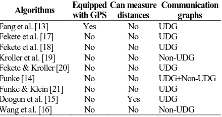
Based on the assumptions made on sensor nodes, we compare the algorithms against the availability of location information, distance information and the communication graphs. Thus, only the geometric algorithm proposed by Fang et al. [13] assumes geographic location information, and only the algorithm developed by Deogun et al. [15] assumes exact distance information. In addition, most of the algorithm assume unit disk graph model [13, 15, 17, 18, 20, 21]. The summary of the assumptions on sensor nodes is presented in Table 2.
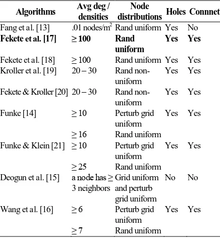
Similarly, we compare our reviewed boundary detection algorithms on WSN conditions. We evaluate several algorithm requirements on networks, such as the minimum average degrees or densities, node distributions, the existence of communication holes and the necessity of connected networks. We summarize and present the assumptions made on networks by the reviewed boundary detection algorithms in Table 3.
Table 1. Boundary detection algorithms against techniques, implementations and results of the algorithms
Algorithms Techniques Implementation Boundary cycles
Fang et al. [13] Geometric Distributed Yes
Fekete et al. [17] Statistical Distributed Yes
Fekete et al. [18] Statistical Distributed Yes
Kroller et al. [19] Topological Distributed Yes Fekete & Kroller [20] Topological Distributed Yes
Funke [14] Topological Centralized No
Funke & Klein [21] Topological Distributed No
Deogun et al. [15] Topological Distributed No
Wang et al. [16] Topological Distributed Yes
Table 2. Boundary detection algorithms against assumptions made on sensor nodes
Table 3. Boundary detection algorithms against assumptions made on networks
Algorithms Avg deg / densities
Node
distributions Holes Connnet
Fang et al. [13] .01 nodes/m2 Rand uniform Yes No
Boundary detection algorithms are better not centralized as they have to rely on a central base station to perform the whole computation. Distributed algorithms can perform best in disconnected networks with low average densities and communication holes. Moreover, location-free algorithms are also preferred, because by not attaching GPS on sensor nodes, the cost to build the network can be reduced.
REFERENCES
1. Stojmenovic, I., 2005, Handbook of Sensor Networks: Algorithms and Architectures. John Wiley & Sons, Inc.
2. Akyildiz, I.F., Su, W., Sankarasubramaniam, Y. and Cayirci, E., 2002, Wireless Sensor Networks: A Survey. Computer Networks, Volume 38, Number 4, pp. 393-422.
3. Mainwaring, A., Polastre, J., Szewczyk, R., Culler, D. and Anderson, J., 2002, Wireless Sensor Networks for Habitat Monitoring. In Proc. 1st ACM Int'l Workshop Wireless Sensor
Networks and Applications (WSNA’02), Volume
4, pp. 88-97.
4. Yu, L., Wang, N., and Meng, X., 2005, Real-time Forest Fire Detection with Wireless Sensor Networks. In Proc. 2005 Int'l Conf. Wireless Communications, Networking and Mobile
Computing (WiMob’05), Volume 2, pp.
1214-1217.
5. Son, B., Her, Y.S., and Kim, J.G., 2006, A Design and Implementation of Forest-Fires Surveillance System based on Wireless Sensor
Networks for South Korea Mountains. Int'l Journal of Computer Science and Network Security, Volume 6, Number 9B, pp. 124-130. 6. Zeng, Y., Murphy, S.Ó., Sitanayah, L., Tabirca,
T.M., Truong, T., Brown, K., and Sreenan, C.J., 2009, Building Fire Emergency Detection and Response Using Wireless Sensor Networks. In Proc. 9th Int'l Conf. Information Technology and
Telecommunications (IT&T’09), pp. 163-170. 7. Gupta, R., and Das, S.R., 2003, Tracking Moving
Targets in a Smart Sensor Network. In Proc. 58th
IEEE Vehicular Technology Conf. (VTC’03
-Fall), Volume 5, pp. 3035-3039.
8. Xu, Y., Winter, J., and Lee, W.C., 2004, Dual Prediction-Based Reporting for Object Tracking Sensor Networks. In Proc. 1st Ann. Int'l Conf. Mobile and Ubiquitous Systems: Networking and
Services (MobiQuitous’04), pp. 154-163. 9. Savvides, A., Han, C.C., and Srivastava, M.B.,
2001, Dynamic Fine-Grained Localization in Ad-Hoc Networks of Sensors. In Proc. 7th Ann. Int'l Conf. on Mobile Computing and Networking
(MobiCom’01).
10. Mao, G., Fidan, B., and Anderson, B.D.O., 2007, Wireless Sensor Network Localization Tech-niques. Computer Networks, Volume 51, Number 10, pp. 2529-2553.
11. Royer, E.M., Melliar-Smith, P.M. and Moser, L.E., 2001, An Analysis of the Optimum Node Density for Ad Hoc Mobile Networks. In Proc. IEEE Int'l Conf. Communications (ICC’01), Volume 3, pp. 857-861.
12. Zhao, F. and Guibas, L.J., 2004, Wireless Sensor Networks - An Information Processing Approach. Morgan Kaufmann Publishers Inc.
13. Fang, Q., Gao, J. and Guibas, L.J., 2006, Locating and Bypassing Holes in Sensor Networks. Mobile Networks and Applications, Volume 11, Number 2, pp. 187-200.
14. Funke, S., 2005, Topological Hole Detection in Wireless Sensor Networks and its Applications. In Proc. 3rd ACM/SIGMOBILE Int'l Workshop Foundations of Mobile Computing
(DIALM-POMC’05), pp. 44-53.
15. Deogun, J.S., Das, S., Hamza, H.S. and Goddard, S., 2005, An Algorithm for Boundary Discovery in Wireless Sensor Networks. In Proc. 12th High
Performance Computing Int'l Conf. (HiPC’05), Volume LNCS 3769, pp. 343-352.
17. Fekete, S.P., Kroller, A., Pfisterer, D., Fischer, S., and Buschmann, C., 2004, Neighborhood-Based Topology Recognition in Sensor Networks. In Proc. 1st Int'l Workshop Algorithmic Aspects of
Wireless Sensor Networks (ALGOSENSORS’04),
Volume LNCS 3121, pp. 123-136.
18. Fekete, S.P., Kaufmann, M., Kroller, A., and Lehmann, K., 2005, A New Approach for Boundary Recognition in Geometric Sensor Networks. In Proc. 17th Canadian Conf. Computational Geometry (CCCG’05), pp. 82-85.
19
.
Kroller, A., Fekete, S.P., Pfisterer, D., and Fischer, S., 2006, Deterministic Boundary Recognition and Topology Extraction for Large Sensor Networks. In Proc. 17th Ann. ACM-SIAM Symp. Discrete Algorithms, pp. 1000-1009.20. Fekete, S.P., and Kroller, A., 2006, Geometry-Based Reasoning for a Large Sensor Network. In Proc. 22nd Ann. Symp. Computational Geometry, pages 475-476.
21. Funke, S. and Klein, C., 2006. Hole Detection or: "How Much Geometry Hides in Connectivity?". In Proc. 22nd ACM Symp. Computational