Testing for asymmetric pricing in the
Canadian retail gasoline market
Rob Godby
a, Anastasia M. Lintner
b,U, Thanasis Stengos
c,
Bo Wandschneider
da
Department of Economics, Uni¨ersity of Wyoming, Laramie, WY, USA b
Department of Economics, Memorial Uni¨ersity of Newfoundland, St John’s, Newfoundland, Canada A1C 5S7
c
Department of Economics, Uni¨ersity of Guelph, Ontario, Canada dData Resource Center, Uni¨ersity of Guelph, Ontario, Canada
Abstract
This paper applies a Threshold Regression model to test for asymmetric pricing in the retail gasoline market in Canada, using weekly data for the period January 1990 to December 1996. We present results for 13 Canadian cities for both premium and regular gasoline. Within the context of an error correction model we test for the presence of asymmetric price behaviour using average changes in crude prices as well as various lags for the change in crude as possible thresholds. We are unable to find any evidence to support this view.Q2000 Elsevier Science B.V. All rights reserved.
JEL classifications:C52; D4; Q40
Keywords:Threshold Autoregressive model; Asymmetric pricing; Price competition; Gasoline
1. Introduction
This paper attempts to determine whether an asymmetric response to unantici-pated positive and negative crude cost shocks can be identified in Canadian retail gasoline price data. Inquires within several countries have focused on the degree,
Ž .
speed and duration of the pass-through of an input crude cost shock to the retail gasoline market. Most often, it is found that the response to a crude cost increase
U
Corresponding author.
0140-9883r00r$ - see front matterQ2000 Elsevier Science B.V. All rights reserved.
Ž .
is quicker and more intense than that of a decrease. Previous studies for the UK and the US have found evidence of this type of asymmetric pricing within their
1 Ž .
markets. Kirchgassner and Kubler 1992 found asymmetry in the opposite direc-
¨
¨
tion; the response to a crude cost decrease was greater than to an increase. There have been several studies of the Canadian gasoline market completed for the Competition Bureau. In each instance, no evidence of an asymmetric pricing
Ž .
pattern was found for example, see Hendricks, 1996 . In this paper we do not
Ž .
attempt to explain the asymmetric adjustment path or lack thereof in response to crude cost increases and decreases; rather, we propose the use of a threshold regression method to explore the short-run asymmetries that may be present in the Canadian market.
Previous studies have been methodologically restrictive in the sense that the
Ž .
short-run response in current retail gasoline price, given an input crude cost shock, was assumed to be dependent only on whether crude costs were rising or falling, and then the authors attempted to identify such a pattern in the data. These studies would therefore be misspecified if mark-up rules were actually described by an alternative relationship, as would be the case if, for example, price
asymmetries were instead triggered by a minimum absolute increase in crude cost.2
In order to address this concern, we apply a Threshold Autoagressive model
ŽTAR , within an error correction framework, to Canadian data. Using several.
possible lagged crude cost]retail price relationships, we attempt to determine
whether an asymmetric pricing pattern in the weekly data for 13 cities can be
distinguished for the period 1990]1996.
We do not find evidence of asymmetric pricing behaviour. This result is not necessarily unexpected, as there are several differences in the Canadian market structure in contrast to the countries considered in the earlier studies. Additionally, some previous studies used gasoline retail price series aggregated over many regional markets while the data used in this study considers regional markets individually. Finally, the frequency of the data in this study is weekly, whereas the
Ž .
other studies were restricted due to data availablity to biweekly or monthly data. The following section motivates in more detail the problem considered. Section 3 describes the partial and full adjustment models used in previous studies. In Section 4, we present the theoretical aspects of the TAR model and explain why its use is the appropriate framework in which to consider our problem. Section 5 describes the data, makes explicit the econometric model used and reports our empirical results. Lastly, Section 6 summarizes and suggests some potential expla-nations for our findings.
1 Ž . Ž . Ž .
Studies for the UK include: Bacon 1991 , Manning 1991 , Reilly and Witt 1998 . Borenstein et al. Ž1997 analysed the US market..
2 Ž .
2. Motivation
With the repeal of the National Energy Program in 1985, world crude oil price volatility was no longer filtered in Canada by the regulated crude oil price regime the program had outlined. As a result, it should be expected that unanticipated crude oil price movements would be reflected in the movement of gasoline prices
observed after the Act’s repeal.3 The fact that the crude oil and gasoline refining
sector in Canada is relatively concentrated } combined with the deregulation of
crude prices } has fostered considerable discussion of the possibility of
non-com-petitive market practices being pursued in the retail gasoline industry.
Concern regarding the state of competition in the industry climaxed in the months leading up to the Persian Gulf War as world crude oil prices reached $US 40 per barrel. Media reports at the time suggested that Canadian gasoline retail prices immediately responded to this shock and, although the crude oil price peak was short-lived, in many centres higher gasoline prices persisted. The Canadian business press and some Canadian politicians began accusing the petroleum industry of taking advantage of world events by immediately passing on input costs to the public as ‘unwarranted’ price increases, taking advantage of world events to increase profits at the expense of the general public. Some groups went as far as suggesting that recent price hikes in the unregulated provinces were the result of too little competition in the industry, and that the federal government should
institute price controls.4 In general, critics claimed that prices were being set
asymmetrically; that world crude price increases were reflected immediately by retail gasoline price increases but that cost decreases took much longer to filter down to prices at the pump. Implicit in the speculation of asymmetric pricing was the assertion that adjustments in retail gasoline prices should reflect changes in crude costs at the time of production in a competitive market. Industry countered these criticisms with assurances that gasoline pricing always reflected input costs and noted that input shocks would not be observed at the gasoline pump until all previously purchased input quantities had been used in the system. As such, retail
gasoline prices follow crude oil prices with approximately a 2-month delay.5 Since
the early 1990s, there have been several investigations by the Canadian Competi-tion Bureau that have attempted to determine whether anti-competitive practices were being pursued in this industry. The most recent national inquiry occurred in
Ž .
May 1996 Competition Bureau, 1997 . Some of these investigations have resulted in trials and convictions; however, evidence of possible asymmetric pricing or collusion has been only circumstantial. As stated in a recent report, ‘For the most part . . . these cases have concerned local markets and isolated incidents. To date,
3
In an attempt to reduce this variation, the eastern Canadian provinces of Nova Scotia and Prince Edward Island instituted full price regulation. Nova Scotia eliminated regulation in July 1991, leaving
Ž Prince Edward Island the only province in Canada still enforcing gasoline price controls Natural
. Resources Canada, 1997c .
4 Ž .
One such group was the Consumer’s Association of Canada. See Fagan 1990 .
5 Ž .
no inquiry has ever produced evidence suggesting that there is a national or
Ž .
regional conspiracy to limit competition’ Competition Bureau, 1997 . Despite these findings, Canadian politicians and media continue to lament the lack of competition in the Canadian market. Such claims have not been limited to Canada,
Ž .
and investigations both formal and informal into similar allegations were made in
the US, the UK, and Germany.6
The uncompetitiverasymmetric pricing assertion includes two aspects of poten-tial differences: short-run vs. long-run adjustments. Whether or not cost changes
Ž
are fully passed on to the final user as would be the case for a constant returns to
.
scale competitive market is of interest in terms of the long-run adjustment. In the short-run, we are interested in differences in the time path of adjustment which will include the lag until and size of the initial response, as well as the duration of response. Previous studies have performed analyses of these issues based on different sample frequencies and periods within several counties.
ln the UK, several authors have considered the question of asymmetric lags in the short-run speed of adjustment of retail gasoline prices relative to world
gasoline prices. For the period of 1982]1989, the Monopolies and Mergers
Commission found that a ‘rockets and feathers’ pattern was apparent in the UK price data. Given that the Commission’s findings were based only on graphical analysis using biweekly data, no evidence could be found to show that this behaviour had been caused by a monopolistic structure in the retail gasoline
Ž .
industry nor that even temporary excess profits had been generated Bacon, 1991 .
Ž . Ž .
Bacon 1991 also tested the UK biweekly retail data more rigorously using a quadratic partial adjustment model to determine whether the data statistically
supported pricing asymmetries between retail and wholesale gasoline prices.7 His
results found evidence that the ‘rockets and feathers’ hypothesis was supported by the data, with the speed of adjustment for retail gasoline prices to product price and exchange rate shocks differing, depending on whether the shock resulted in an
Ž .
input price increase or decrease. Bacon 1991 also tested for the pass-through of crude cost changes to the retail price in the long-run and found evidence that changes in the exchange rate adjusted crude cost are fully passed on to retail prices.
Employing a less restrictive method of modeling the lag adjustment process than
Ž . Ž . Ž .
Bacon 1991 , Manning 1991 , and Reilly and Witt 1998 tested for an asymmetric short-run adjustment with an error correction term for the long-run relationship. The short-run adjustment in each case is tested using interactive dummy variables for crude oil price increases with the change in crude oil price. Both studies make
Ž .
use of monthly data; Manning 1991 for the period 1973]1988 and Reilly and Witt
Ž1998 for the period 1982. ]1995. Both find the pass-through is incomplete;
how-ever, the long-run relationship is very different in each of the two cases. Manning
6 Ž . Ž . Ž .
Studies for the UK include: Bacon 1991 , Manning 1991 , Reilly and Witt 1998 . Kirchgassner and¨
Ž . Ž .
Kubler 1992 have considered the German market. Borenstein et al. 1997 analysed the US market.¨ 7
Ž1991 estimates a 7% pass-through of crude costs while Reilly and Witt 1998 find. Ž .
the rate to be 58%. This difference in the long-run relationship may be attributed
Ž .
to the fact that Reilly and Witt 1998 incorporate changes in the exchange rate
Ž .
while Manning 1991 does not.
Ž .
For the Federal Republic of Germany, Kirchgassner and Kubler 1992 use a
¨
¨
monthly average time series for the period 1972]1989 to test for any short-run
asymmetries and long-run pass-through. In addition, they test for structural con-stancy over the period to determine if the market is becoming more competitive
over time. They offer an additional explanation for short-run asymmetries } that
there may be a politico-economic response on the part of petroleum distributors to hesitate when crude costs are rising and thus avoid allegations of uncompetitive or consumer gouging pricing. No such incentive would be in place when crude cost are falling. Thus, one could expect the response to a crude cost increase to be smaller
Ž .
than the response to a crude cost fall. Kirchgassner and Kubler 1992 find
¨
¨
evidence for this politico-economic asymmetry using a full adjustment error
correc-Ž
tion model. They tested a restricted different independent variables representing
.
crude cost increases and decreases against the unrestricted symmetric lagged response to any crude cost change. It does not appear that a time trend was
Ž .
included in the estimation. Kirchgassner and Kubler 1992 found that there was
¨
¨
full pass-through in the long-run and that the market appears to be more
Ž .
competitive over time estimated two samples, the 1970s and 1980s .
Ž .
Using data from the eastern US, Borenstein et al. 1997 have tested for asymmetric pricing patterns between retail gasoline prices and world crude oil prices. They determined that US retail gasoline prices do respond more quickly to
input price increases than decreases using biweekly data.8 By defining the
interme-diate stages of the gasoline production process from refining to retail, they also identified the intermediate transactions where asymmetric mark-ups could occur.
Ž .
Using additional American price data available at all stages of production ,
Ž .
Borenstein et al. 1997 found significant asymmetries between changes in crude oil prices and gasoline commodity spot prices and also between gasoline terminal prices and retail prices. No such asymmetry in the mark-up from spot prices to terminal prices was observed.
To determine whether an asymmetric relationship is present between changes in crude costs and Canadian retail gasoline prices, we employ an error correction model where short-run dynamics are linked to long-run equilibrium behaviour. We
Ž .
hypothesize that long-run retail gasoline prices net of taxes should reflect crude costs, but allow that in the short-run this relationship may be less tight, as input cost adjustments may occur in a lagged manner. We are fortunate to have weekly data and, unlike the other studies mentioned, can capture the very short-run asymmetries. We employ a number of changes in methodology relative to the
8
Assuming that a typical consumer purchases 10 US gallons of gasoline per week, the authors estimated that a $0.05 increase in the price of a gallon of crude oil costs the consumer $1.30 more over the life of
Ž
the price adjustment than the cost saving generated by an equal crude oil price decrease Borenstein et .
previous literature. Gasoline price data used here is regional, as opposed to the
Ž . Ž .
aggregate data used in Kirchgassner and Kubler 1992 , Borenstein et al. 1997 ,
¨
¨
and the crude costrgasoline price relationship is estimated in several centres, as
Ž .
opposed to the single centre studied in Bacon 1991 . Additionally, the econometric method employed is less restrictive than that used in either of the previous studies. We fully describe our method, while reviewing and comparing it to previous methods, in the following section.
3. Partial and full adjustment models
One model used to explain the response of gasoline prices to input cost shocks is
the partial adjustment model. The current price yt, is set at last period’s price with
an adjustment for any differences between last period’s price and the target level,
yU
, according to the following relationship: ty1
Ž . Ž U
. Ž .
ytsyty1q 1yf yty1yyty1 q«t 1
wherefis the speed of adjustment. From an equilibrium where y syU
, a shock ty1 t
to yU
will result in an infinitely slow adjustment toward the new equilibrium if ty1
fs1 and an instantaneous adjustment to the new target if fs0. Given that
Ž
crude cost is the single determining factor in gasoline prices Natural Resources
.
Canada 1997b , it is assumed that the target price is the long-run equilibrium price,
U Ž .
y sc0qc1cq«, 2
Ž .
wherec0 is other costs and margins which we consider to be essentially constant ,
c is the crude cost, and c1, represents the proportion of the crude cost which is
passed through to the retail gasoline price. In this long-run relationship, whether
or not c1, is equal to one will depend on the market under study.
Ž .
Bacon 1991 observed that a partial adjustment would not allow for a proper assessment of the asymmetric responses to two separate shocks in the target price
Ži.e. an unanticipated crude cost decrease followed by an unanticipated crude cost
.
increase unless the researcher were able to split the sample into the appropriate sub-samples. Since it is not possible, a priori, to know the appropriate sample split,
Ž .
Bacon 1991 proposed the following quadratic partial adjustment mechanism,
2
U U
Ž . Ž . Ž .
ytsyty1qa0 yty1yyty1 qa1 yty1yyty1 q«t, 3
where the hypothesis that a1s0 reflects a symmetric pricing response. If botha0
and a1, are greater than zero, the response to a crude cost increase will be more
rapid early on than a crude cost decrease. If a0-0 and a1)0, the response is
Ž .
more rapid to a crude cost decrease. Bacon 1991 found the former to be true in the UK.
all periods after a shock and the asymmetry must become proportionately larger with an increase in the difference between current and long-run equilibrium prices
ŽBorenstein et al., 1997 . Subsequently, an asymmetric full adjustment model is.
proposed,
where p is the number of lags over which the shock is felt, Dcq are the positive
tyk
changes in the crude cost, and Dcy are the negative changes in the crude cost. In
tyk
Ž .
order to ensure that the error term is white noise, Borenstein et al. 1997 included lagged changes in past gasoline prices in their estimation. After estimating the crude cost series by instrumental variables, the second stage involved estimating,
p
The coefficients on the lagged price level and the lagged crude oil price can be
used then to uniquely determine the pass-through coefficient, c1.
Ž .
Kirchgassner and Kubler 1992 adopted an approach which is similar to Boren-
¨
¨
Ž . U
stein et al. 1997 . For both models, the long-run price, yt, was estimated in the
Ž .
first stage using Eq. 2 . The second stage involved estimating an unrestricted and restricted model,
regression and is referred to as the error correction term.
To motivate the differences between the full adjustment error correction model and the approach adopted in this paper, consider a full adjustment model with a lag length of only one period. All else equal, the short-run response in current retail price will be determined by a change in the current crude cost only. A symmetric response would be represented by the dashed line in Fig. 1. The solid line represents an asymmetric response such that the price is adjusted upwards by a larger proportion of the crude cost change when crude prices are increasing than
Ž q y.
when decreasing u0)u0 . Suppose that the actual response follows a more
Fig. 1. ] ] ]symmetric}asymmetric.
X
Ž .
Dy1sa D0 c0, Dc0Fg 8
X
Ž .
Dy1sd D0 c0, Dc0)g 9
In Fig. 2, the threshold formulation is the darker solid line. The response to a crude cost change is to increase the retail price byaX0Dc0 for all changes in crude cost less than or equal to g. When the crude cost changes by more than g, the response is to change the retail price by dX0Dc0, where aX0-dX0.
The asymmetric full adjustment model allows that there is a different response to crude cost increases and decreases, but it requires that the threshold for this
asymmetric response be a zero change in the crude cost and does not allow for a dynamic threshold effect. The Threshold Regression model does not impose these restrictions.
( ) 4. The Threshold Autoregressive TAR model
Ž .
In this paper we will follow Hansen 1998 who suggests a bootstrap procedure to test the null hypothesis of a linear formulation against a Threshold Autoregressive
ŽTAR alternative. We employ the TAR model to answer the following questions:.
Is there evidence of asymmetric pricing in major Canadian markets over the period January 1990 to December 1996? Asymmetric pricing is tested for in both regular and premium gasoline markets for 13 Canadian cities.
Ž .
The typical linear Autoregressive AR model is based on a linear mechanism that relies on information that is contained in the autocovariance function of the time series, a condition that imposes strong symmetry requirements on the dy-namics of the estimated model. In other words, the propagating linear mechanism in an AR specification results in uncorrelated impulses, so that deviations from below will not systematically differ from the ones from above the trend.
On the other hand a non-linear model that does not impose a symmetry restriction would require that additional information about moments beyond autocovariances are important to estimate the model. This lack of symmetry restriction is a distinguishing feature of the non-linear time series model that we employ in this paper. The TAR model allows for non-symmetrical treatments of deviations from trend and as such has found a number of useful applications in economics. In particular it has been applied to explore asymmetric behaviour of macroeconomic time series over the business cycle, see Granger and Terasvirta
¨
Ž1993 , Potter 1995 . More recently Hansen 1998 has provided the non-stan-. Ž . Ž . Ž.
dard asymptotic distribution theory for estimating and testing of the TAR model for both cross-section and time series applications.
Ž .
In this paper we apply Hansen’s 1998 results to study the asymmetric response of gasoline price changes with respect to past changes in gasoline prices and crude oil costs.
The TAR model can he expressed as follows. Let the data be given yt, xt, 4n
qt ts1, where yt and qt are observations on the dependent variable and the threshold variable that splits the sample into different groups, respectively, and xt is a p=1 vector of independent variables. The threshold variable qt may be part of xt. It may also be the case that xt contains lagged values of the dependent variable. The model is then given by
T Ž .
ytsxtb1q«t, qtFg 10
T Ž .
The model can be written in a single equation form, by defining the dummy change between sample groups. In matrix notation the above model can be written as follows. Define Y and u to be the n=1 vectors of the observations on the dependent variable and error term, respectively, and let X and Xg be the n=p
T T Ž .
matrices with respective rows xt and xt. Then Eq. 12 can be written as
Ž .
YsXbqXguqu 13
Ž . Ž .
The regression parameters b,u,g can be estimated using least squares LS . The
Ž .
sum of squared errors SSE function is minimized to give the values of the LS estimates. The SSE function is given by
T
Sn b,u,g . The objective function is non-linear and discontinuous in the parameter
g and therefore there is no closed form solution. However, for a given value of g, say gU
, the SSE is linear in b and u. Hence we can obtain by Ordinary Least
U U
ˆ
Uˆ
UHansen 1998 has provided an algorithm that searches over possible values ofg
using conditional OLS regressions based on a sequential search over all gsqi, for
Ž .
is1,...n. The value of gthat minimizes the function Sn g will be the LS estimate,
ˆ
Ž .ˆ
Ž .g. Similarly, the LS estimates of b and u will be given by b g. and u g. . The
ˆ
ˆ
ˆ
asymptotic distribution of the above LS estimators is derived under certain condi-tions that weaken the threshold effect as the sample size increases and therefore result in an asymptotic distribution free of nuisance parameters for the threshold estimator g
ˆ
.9An important hypothesis of interest is whether the TAR model is statistically significant relative to a simple linear specification. The null hypothesis in this case describes the simple linear specification and is expressed as
H :0 b1sb2
Devising a test for the above null hypothesis runs into the difficulty that the threshold parameter g is not identified under H0. This is a problem that is
9 Ž .
For identifiability purposes, Hansen 1998 also suggests to trim the bottom and top 15% quantiles of the threshold variable to rid the model of possible heteroskedastic error effects. For further details of
Ž .
analyzed in the literature in different contexts by Davies 1977, 1987 , Andrews and
Ž . Ž . Ž .
Ploberger 1994 , Kim et al. 1995 , Hansen 1996 . In this paper we will follow
Ž .
Hansen 1998 who suggests a bootstrap procedure to test the above null hypothe-sis of a linear formulation against a TAR alternative. The test is robust to
10 Ž .
heteroskedastic errors. Monte Carlo evidence provided by Hansen 1998 sug-gests that the proposed test has good small sample properties.
5. The data and empirical results
The data were gathered from Department of Natural Resources publications:
Ž
Petroleum Product Pricing Report and Crude Oil Pricing Report Natural
Re-.
sources Canada, 1990]1996 . The gasoline prices are collected on Tuesday of each week between the period from January 1990 to December 1996 and for each of 13
Ž .
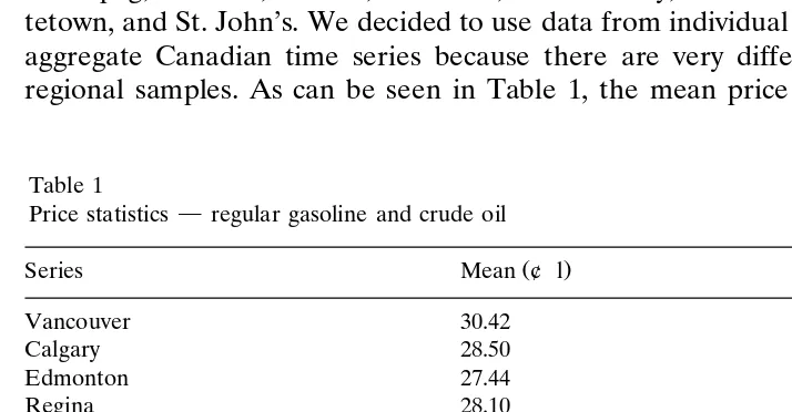
major centres across Canada for a total of 366 observations per city. In each centre, only self serve stations are surveyed and the majority of the stations are brand names such as Esso, Shell, and Petro-Canada. The gasoline prices are exclusive of taxes. The cities tested are: Vancouver, Calgary, Edmonton, Regina, Winnipeg, Toronto, Ottawa, Montreal, Quebec City, Saint John, Halifax, Charlot-
´
´
tetown, and St. John’s. We decided to use data from individual cities rather than an aggregate Canadian time series because there are very different patterns in the regional samples. As can be seen in Table 1, the mean price for regular gasolineTable 1
Price statistics}regular gasoline and crude oil
Ž .
To carry out the empirical analysis we have adapted a GAUSS program written by Hansen, used to Ž .
Table 2
Price statistics}premium gasoline
Ž .
City Mean ¢rl S.D.
Vancouver 37.30 3.590
Calgary 35.50 4.160
Edmonton 34.30 4.110
Regina 34.90 4.260
Winnipeg 36.90 3.870
Toronto 34.00 3.540
Ottawa 36.40 3.300
Montreal´ 36.10 4.390
Quebec City´ 36.50 4.010
Saint John 38.60 2.720
Halifax 36.70 3.760
Charlottetown 37.40 2.560
St. John’s 39.04 3.625
Canada 35.92 3.089
varies from a low of 26.99¢rl in Edmonton to a high of 34.42¢rl in Charlottetown. The mean for the aggregate Canadian series is 29.11¢rl. The variation in the data is also quite different by region. Only three cities have a smaller standard deviation than the Canadian average; however, several have significantly more variation. Similar conclusions can be reached regarding the premium prices series, as indicated in Table 2.
Ž .
Crude oil prices were obtained for two locations, Edmonton Par and Montreal
´
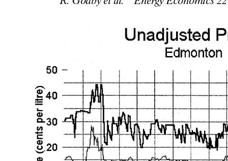
ŽBrent ..11 The observation for Tuesday of each week was used. In Table 1, theFig. 4. —Regular Gasoline}Edmonton Par
mean standard deviations of the two series are reported. Only Charlottetown has less variation than the crude oil price, due to the fact that the gasoline prices continue to be regulated in that city. As can be seen in Fig. 3, the two crude oil price series are almost identical, with the Montreal Brent price generally above the
´
Edmonton Par price. Figs. 4]7 present the plots of the price series for Canada, Toronto, Edmonton and Saint John, respectively. On each diagram there is also a plot of the appropriate crude oil price series.
Fig. 6. —Regular Gasoline}Edmonton Par.
6. Seasonality, unit roots and cointegration
Before starting our analysis we deseasonalized the data. The process involved regressing the crude oil prices and the gasoline prices on a series of 53 weekly dummies.12 The residuals represent the deseasonalized series. We will denote by Y
the deseasonalized gasoline price and by C the deseasonalized crude price. We first tested each series for unit roots. We used the ADF test where we
Ž .
regressed the change in price premium, regular, crude on a constant, time trend a lagged value of the price and eight weekly lags of the change in price. In the majority of cases we find evidence for a unit root in these series manifested with a value of the coefficient of the lagged price variable not statistically different from
Ž .
zero using the standard tables for the ADF test see Hamilton, 1994 . This finding
Ž . Ž .
is consistent with Borenstein et al. 1997 and Kirchgassner and Kubler 1992 .
¨
¨
Therefore, we conclude that all prices are first difference trend stationary.
We then tested the premium and regular gas prices to see if they were cointegrated with the crude prices. We use the EnglerGranger test where the residuals from an OLS regression of the gasoline price on a constant and the crude price are tested for a unit root using the ADF test. As in the case of the single price series we use eight lags of the change in residuals in order to induce white noise error terms in the ADF regressions. We used the critical values of
Mackin-Ž .
non 1991 . We find strong evidence against the null hypothesis of no cointegration
11
Following the format of other studies, we estimated our models using Edmonton Par for all cities. We then estimated the model for cities in Ontario and east using Montreal Brent. There was no significant´ difference in our results.
12
Fig. 7. —Regular Gasoline}Montreal Brent
in favor of the cointegration alternative. We therefore proceed as if the gasoline and crude prices are cointegrated.
7. Error correction TAR model
Ž .
As in Borenstein et al. 1997 , in order to take into account the long-run relationship between the crude prices and the retail prices we introduce an error correction term into our model. To achieve this we regress the levels of prices on the level of crude with an intercept term. Since we find strong evidence that the series are cointegrated we introduce the lagged residual series from estimating Eq.
Ž .2 to the TAR model as the error correction variable. Consequently, the estimated model is written as
p X
DYt,isa0qa1Zty1 ,iq
Ý
a Dk Ctyk,iq«i,t, qi-g, is1, . . . , 13; ks0Ž .
ts1, . . . , 366. 15
p X
DYt,isd0qd1Zty1 ,iq
Ý
d Dk Ctyk,iq«i,t, qiGg, is1, . . . , 13; ks0Ž .
ts1, . . . , 366. 16
information criterion. Although it varied from city to city, eight lags turned out to be the preferred choice. Consequently, we use the average of the last eight crude
Ž
price changes as a threshold indicating average changes over the previous 2
.
months as well as individual lagged crude changes. We report the results for four of these lags for each city and crude price choice.13 We assume that the markets
for each city are independent and, as such, we do not allow for possible dependen-cies of the error structures between different cities.
Ž . Ž .
Eqs. 5 and 6 above provide a less restrictive formulation than what has been traditionally estimated in the literature. By using the partial or full adjustment models, researchers impose a threshold at zero. They then proceed to estimate possible asymmetries that arise from differential responses of gasoline price
Ž
changes to positive and negative changes in crude prices see Borenstein et al.,
.
1997 . Furthermore, we provide a direct test for asymmetric behaviour around the estimated threshold. The null hypothesis of no asymmetry is expressed as
H0:asd
Ž X X
.T Ž X X
.T
whereas a0, a1, a1, . . . , ak andds d0, d1, d1, . . . , dk . The test we use is based on bootstrap critical values of a Wald type heteroskedasticity-consistent test
Ž .
of the null hypothesis above against a TAR alternative see Hansen, 1997 . The results from the TAR model are presented in Tables 3]6. Tables 3 and 5 contain the results for premium and regular gasoline, respectively, using Edmonton par as the crude cost. For cities located east of, and including, Toronto we ran the
Ž
model using Montreal Brent as the crude cost see Tables 4 and 6 for premium and
´
.regular gasoline, respectively . The thresholds AVGE and AVGM are the average change in the crude oil price over the previous eight periods for Edmonton par and Montreal Brent, respectively. DC1 is a threshold representing a one period lagged
´
change in the crude oil price. DC2, DC3, and DC4 have similar interpretation, for the two, three and four period lagged thresholds, respectively. The instances where the P-value lies below 0.05 are highlighted in bold and represent rejections of the null hypothesis, where the null hypothesis is that there is no significant threshold
Žno asymmetry . This rejection of the null occurs so infrequently that we can safely.
argue that asymmetry is not present in the Canadian retail gasoline market. These results support the results obtained in the studies by the Competition Bureau, but
Ž .
differ from the results obtained by Borenstein et al. 1997 for the US, by
Ž . Ž . Ž .
Kirchgassner and Kubler 1992 in Germany, and by Bacon 1991 , Manning 1991 ,
¨
¨
Ž .
and Reilly and Witt 1998 for the UK. We will outline some of the reasons why this may be the case in the next section.
13 Ž .
In the TAR formulation of the model we only report results that correspond to Eq. 4 of the full Ž . Ž .
adjustment model, see Eqs. 11 and 12 above. However, we also looked at extensions of the type given
Ž . Ž .
Table 3
a
Ž .
P-values Premium Gasoline}Edmonton Par
City AVGE DC1 DC2 DC3 DC4
Vancouver 0.3420 0.8610 0.1990 0.3640 0.3370
Calgary 0.0560 0.7590 0.8620 0.1770 0.6040
Edmonton 0.4410 0.0610 0.8470 0.1970 0.1630
Regina 0.8100 0.6920 0.2220 0.3010 0.5370
Winnipeg 0.5340 0.6040 0.0170 0.1620 0.6470
Toronto 0.3790 0.3470 0.3160 0.2930 0.7480
Ottawa 0.2630 0.0650 0.1160 0.7180 0.0730
Montreal´ 0.1100 0.9690 0.1960 0.2090 0.2710
Quebec City´ 0.1240 0.1220 0.0520 0.0820 0.6590
Saint John 0.9920 0.3140 0.1400 0.2580 0.7730
Halifax 0.0950 0.3110 0.1440 0.2450 0.8240
Charlottetown 0.7990 0.9060 0.8010 0.8960 0.3430
St. John’s 0.9870 0.0870 0.5380 0.3700 0.7430
a Ž .
The bold values indicate a rejection of the null hypothesis no threshold .
8. Summary
Ž .
In this paper we follow Hansen 1998 who suggests a bootstrap procedure to
Ž .
test the null hypothesis of a linear symmetric formulation against a TAR alternative. We employ the TAR model to answer the following questions: Is there evidence of short-run asymmetric pricing in major Canadian retail gasoline mar-kets over the period January 1990]December 1996? Asymmetric pricing is tested for in both regular and premium gasoline markets for 13 Canadian cities.
The major contribution of this paper is in the application of the TAR model to this particular question. Previous studies restricted the threshold to be zero and it has been suggested in the context of the Canadian market that this may not necessarily be the case. It is possible that the threshold lies at some positive value
Table 4
a
Ž .
P-values Premium Gasoline}Montreal Brent´
City AVGM DC1 DC2 DC3 DC4
Toronto 0.7560 0.3270 0.2330 0.0540 0.4930
Ottawa 0.3290 0.6110 0.0360 0.8500 0.2730
Montreal´ 0.1300 0.8110 0.5500 0.0830 0.7490
Quebec City´ 0.1210 0.0570 0.0670 0.2170 0.3830
Saint John 0.7660 0.3790 0.3930 0.8490 0.4370
Halifax 0.0140 0.1320 0.3970 0.0240 0.4300
Charlottetown 0.7130 0.7560 0.6910 0.5000 0.7700
St. John’s 0.5800 0.0280 0.4700 0.1470 0.2720
a Ž .
Table 5
a
Ž .
P-values Regular Gasoline}Edmonton Par
City AVGE DC1 DC2 DC3 DC4
Vancouver 0.2970 0.7670 0.1510 0.3230 0.2900
Calgary 0.0680 0.8120 0.8810 0.1680 0.7780
Edmonton 0.1990 0.1800 0.7480 0.1810 0.2670
Regina 0.4030 0.6290 0.1760 0.3620 0.6740
Winnipeg 0.4860 0.7310 0.0140 0.0650 0.4980
Toronto 0.3080 0.5200 0.2700 0.2690 0.9240
Ottawa 0.2600 0.1200 0.1240 0.8920 0.3010
Montreal´ 0.1300 0.9830 0.5480 0.3450 0.4040
Quebec City´ 0.3080 0.4640 0.0260 0.2750 0.4340
Saint John 0.6950 0.1040 0.3330 0.5650 0.4950
Halifax 0.5530 0.3620 0.1500 0.5230 0.8240
Charlottetown 0.8890 0.9510 0.8760 0.9160 0.3780
St. John’s 0.6720 0.0190 0.3250 0.5200 0.8070
a Ž .
The bold values indicate a rejection of the null hypothesis no threshold .
or it may be that the asymmetric behaviour is not triggered until a certain change in crude is felt in some fixed time period. Using the TAR model within an error correction framework and choosing the eight period average change in crude allows us to test for these asymmetries.
Unlike the US, UK or German studies we find no evidence of asymmetric behaviour. This is not unexpected as this is similar to results obtained by the Competition Bureau. Several reasons for these differences have been alluded to. In general they can be grouped into those related to market structure, those related to the data and those related to the methodology.
The first possible explanation is related to differences in market structure between Canada and other countries. In particular, the Canadian industry con-trasts quite remarkably with the US industry. Canada has twice the number of
Table 6
a
Ž .
P-values Regular Gasoline}Montreal Brent´
City AVGM DC1 DC2 DC3 DC4
Toronto 0.7020 0.2650 0.1350 0.0610 0.5940
Ottawa 0.6310 0.5040 0.0960 0.6790 0.6150
Montreal´ 0.1570 0.8040 0.9440 0.1620 0.8520
Quebec City´ 0.1040 0.0860 0.4330 0.2760 0.4190
Saint John 0.4020 0.0450 0.2710 0.7090 0.3380
Halifax 0.1250 0.1780 0.2460 0.3900 0.1650
Charlottetown 0.7980 0.4810 0.5780 0.4620 0.7620
St. John’s 0.6400 0.0190 0.6540 0.2180 0.8630
a Ž .
service stations per capita operating at half the level compared to the US.14
Gasoline consumption per vehicle has fallen 3.5 times more in Canada than in the
Ž .
US since the 1980s Industry Canada, 1996 . Suggested reasons for this latter difference are higher taxes and average fuel efficiencies in Canada.15 Finally,
Ž .
Canadian retail margins refinery gate price to pump price have fallen by more than 50% since the 1980s, and are relatively low when compared to the US margins.16 All these factors might suggest that the Canadian market is quite
different than the US market and in turn we see the difference in responsiveness of retail prices to changes in crude.
A second reason for the difference in results between other studies and this paper lies with the data. Data sets of different frequency, periodicity, and level of aggregation were used in each other cited studies. Ignoring the period issues, only this study is able to use weekly data. Other studies were restricted to biweekly or monthly data. This is of concern if the short-run adjustment lag is shorter than the
Ž . Ž .
sample frequency. Both Bacon 1991 , and Borenstein et al. 1997 mention this concern. With weekly data, we suspect that the short-run adjustment lag can be properly captured in the analysis. Another potential difference may lie in the
Ž .
different levels of aggregation in the data. In our analysis, each region city was considered independently, while in the US and Germany, the gasoline price data was an average of potentially distinct regions.17 Considering the nature of the
Canadian refining and distribution network it may be a strong assumption to impose a consistent adjustment process across all cities. It is not clear whether regional symmetric responses to a crude cost shock with differing adjustment lags will show up as symmetric responses in the aggregate or whether regional asymme-tries will come through in the aggregate. This is left for future research.
The final difference between the study relates to the methodology. It is our view that the TAR model is better suited to this analysis, than either of the previously used adjustment models. Both are restrictive in that the threshold is centred around zero and the dynamic response to cumulative shocks cannot be captured.
References
Andrews, D.W.K., Ploberger, W., 1994. Optimal tests when a nuisance parameter is present only under the alternative. Econometrica 61, 821]856.
14 Ž .
Sales were 5300 lrday in Canada vs. 10 000 lrday in US Industry Canada, 1996 .
15 Ž
As of March 1997, taxes in Canada average 28.7¢rl vs. 15.1¢rl in US Natural Resources Canada, .
1997a . The lower fuel efficiency in the US is said to be the result of the fact that turnover in the
Ž .
Canadian ‘fleet’ is faster than in the US Industry Canada, 1996 .
16
As of March 1997, the gross margin was 14.7¢rl in the US, accounting for 31% of the pump price, and
Ž .
only 14.2¢rl in Canada, accounting for 23% of the pump price Natural Resources Canada, 1997a .
17 Ž .
In the US study the data was an average over 33 cities Borenstein et al. 1997 and in the German
Ž .
Bacon, R.W., 1991. Rockets and feathers: the asymmetric speed of adjustment of UK retail gasoline prices to cost changes. Energy Econ. 13, 211]218.
Borenstein, S., Cameron, C.A., Gilbert, R., 1997. Do gasoline prices respond asymmetrically to crude oil price changes? Q. J. Econ. 112, 305]339.
Competition Bureau, 1997. Discontinued inquiries concerning Canada’s gasoline industry, Press Re-lease, Ottawa.
Davies, R.B., 1977. Hypothesis testing when a nuisance parameter is present only under the alternative. Biometrica 64, 247]254.
Davies, R.B., 1987. Hypothesis testing when a nuisance parameter is present only under the alternative. Biometrica 74, 33]43.
Fagan, D., 1990. Gas hikes Moderate: Epp. Globe and Mail 16 October 1990.
Granger, C.W.J., Terasvirta, T., 1993. Modelling Non-linear Economic Relationships. Oxford University¨ Press, Oxford.
Hamilton, J.D., 1994. Time Series Analysis. Princeton University Press, Princeton.
Hansen, B.E., 1996. Inference when a nuisance parameter is not identified under the null hypothesis. Econometrica 64, 413]430.
Hansen, B.E., 1998. Sample splitting and threshold estimation Working Paper no. 319, 1996}revised 1998, Department of Economics, Boston College.
Hendricks, K., 1996. Analysis and opinion on retail gas inquiry, an independent study prepared for the Director of Investigation and Research, Competition Bureau, Canada.
Industry Canada, 1996. Sector Competitiveness Frameworks: Petroleum Products. Canada.
Kim, R., Li, Q., Naiman D., Stengos, T., 1995. On Hotellings’s approach to hypothesis testing when a
Ž .
nuisance parameter is only present under the alternative manuscript , Department of Economics, University of Guelph.
Kirchgassner, G., Kubler, K., 1992. Symmetric or asymmetric price adjustments in the oil market: an¨ ¨ empirical analysis of the relations between international and domestic prices in the Federal Republic of Germany, 1972]1989. Energy Econ. 14, 171]185.
Ž . Mackinnon, J., 1991. Critical values for cointegration tests. In: Engle, R.F., Granger, C.W.J. Eds. ,
Long-Run Economic Relationships: Readings in Cointegration. Oxford University Press, Oxford. Manning, D.N., 1991. Petrol prices, oil price rises and oil price falls: some evidence for the UK since
1972. App. Econ. 23, 1535]1541.
Natural Resources Canada, 1997a. Canada vs. US Average Retail Price, Doc no. 36900. Natural Resources Canada, 1997b. Pump Price Components, Doc no. 36100.
Natural Resources Canada, 1997c. Petroleum Product Documents Methodology and Data Sources. Ž Natural Resources Canada, 1990]1996. Petroleum Product Pricing Reports}Regular Gasoline Doc
. Ž
no. 36190 to Doc no. 36196 , Petroleum Product Pricing Reports }Premium Gasoline Doc no.
. Ž .