q
We are grateful to Andy Abel, Janice Eberly and Nick Souleles for helpful conversations on this topic and to two anonymous referees and seminar participants at Carnegie Mellon, CUNY-Baruch College, Duke, HEC, Hong Kong University of Science and Technology, McGill, Northwestern, University of Hong Kong, University of Mississippi, University of Pennsylvania and Washington University for comments.
*Corresponding author. Tel.: 215-898-8290; fax: 215-898-6200.
E-mail address:[email protected] (D. Cuoco) 24 (2000) 561}613
Optimal consumption of a divisible
durable good
qDomenico Cuoco
!
,
*
, Hong Liu
"
!The Wharton School, University of Pennsylvania, Philadelphia, PA 19104, USA "Olin School of Business, Washington University, St. Louis, MO 63130, USA
Received 1 April 1998; accepted 1 January 1999
Abstract
We examine the intertemporal optimal consumption and investment problem in a continuous-time economy with a divisible durable good. Consumption services are assumed to be proportional to the stock of the good held and adjustment of the stock is costly, in that it involves the payment of a proportional transaction cost. For the case in which the investor has an isoelastic utility function and asset prices follow a geometric Brownian motion, we establish the existence of an optimal policy and provide an explicit representation for the value function. We show that the investor acts so as to maintain the ratio of the stock of the durable to total wealth in a"xed (nonstochastic) range and that the optimal investment policy involves stochastic portfolio weights. The dependence of the optimal policies on the parameters of the model is also discussed. ( 2000 Elsevier Science B.V. All rights reserved.
JEL classixcation: D11; D91; G11; C61
Keywords: Durable goods; Adjustment costs; Singular stochastic control
1. Introduction
This paper studies, in a continuous-time economy with constant price coe$ -cients, the intertemporal optimal consumption and investment problem of an in"nitely lived investor with an isoelastic utility function for the services pro-vided by a perfectly divisible durable good. The consumption services propro-vided by the durable good are assumed to be proportional to the current holdings of the good (net of depreciation), and thus depend on past purchasing decisions. Investments in the durable good are reversible, but a proportional transaction cost has to be paid whenever the good is bought or sold. We allow for di!erent transaction cost rates on purchases and sales.
In the absence of transaction costs, the solution to the problem we study can be easily obtained through a straightforward change of variables from the classical model with a perishable good (Merton, 1971). The investor would continuously adjust the stock of the durable good so as to maintain the marginal utility of consumption equal to the marginal utility of wealth. With the prices of risky assets following geometric Brownian motions, this amounts to keeping a constant fraction of wealth invested in the durable. Similarly, the optimal portfolio policy would involve constant weights.
In the presence of transaction costs, adjusting the stock of the durable continuously would lead to incurring in"nitely large transaction costs. There-fore, the stock of the durable is adjusted only infrequently: transaction costs introduce a wedge between the marginal utility of consumption and the mar-ginal utility of wealth, and the optimal consumption policy involves possibly a discrete change (jump) in the initial stock of the durable, followed by the minimal amount of transactions necessary to maintain the fraction of wealth invested in the durable in a given constant range. The optimal portfolio policy involves investing in the same portfolio of risky assets (the mean-variance e$cient portfolio) as in the Merton case (no transaction costs), but the fraction of wealth allocated to stocks becomes stochastic.
1In their analysis of optimal portfolio policies in the presence of proportional transaction costs, Shreve and Soner (1994, Remark 11.3) provided a su$cient (but not necessary) condition for the optimal fraction of wealth invested in the stock to be uniformly lower than what would be optimal in the absence of transaction costs.
purchases are irreversible, we provide a closed-form expression for the bound-aries of the optimal consumption range and for the value function.
As expected given the nature of the problem (cf."ksendal, 1997), we"nd that small transaction costs can induce large deviations from the amount of durable consumption that would be optimal in the Merton case. The extent of these deviations depends critically on the depreciation rate of the durable good: the optimal policy for short-lived durables involves much more frequent purchases than the one for longer-lived durables. The boundaries of the optimal range for the fraction of wealth invested in the durable are not necessarily monotonic functions of the transaction cost rates, and the fraction of wealth invested in the durable good can be uniformly (i.e., throughout the optimal range) lower than what would be optimal in the Merton case, due to additional savings by the investor to meet future transaction costs. We provide a simple necessary and su$cient condition on the parameters of the model for this to happen.1
We also show that the optimal proportional investment in the durable good converges to a steady-state distribution, which we obtain in closed form. Numerical computations show that, even in cases where the size of the no-transaction region is monotonically increasing in the no-transaction cost rates, the steady-state average investment in the durable is always monotonically decreas-ing in the transaction cost rates.
While transaction costs in the market for the consumption good can induce large deviations of the holdings of the good from the Merton case, deviations of the fraction of wealth invested in risky assets are by comparison more limited. We show that this fraction is always higher than in the Merton case when the investor's wealth is high relative to the current stock of durable (i.e., immediately before or after a purchase), and is always lower when the investor's wealth is low (i.e., immediately before or after a sale). As a result, the investor can behave in either a more or a less risk-averse manner than in the absence of transaction costs, depending on his current wealth and durable holdings, even though the steady-state average investment in stocks is monotonically decreasing in the transaction cost rates. Since two-fund separation holds, the standard CAPM would characterize equilibrium prices in this economy. On the other hand, the consumption-based CAPM (CCAPM) would fail to hold due to the possible divergence between the marginal utility of consumption and the marginal utility of wealth.
2In comparing the model with proportional adjustment costs to the one with"xed costs, it may also be worth pointing out that the solution for the former model is much easier to compute numerically and, as we show in the paper, can be reduced to"nding the zero of a continuous real-valued function that changes sign at the boundaries of a given "nite interval. It is thus straightforward to implement numerical solution algorithms that always converge.
Grossman and Laroque (1990) consider an economy similar to ours, but in which the durable good comes in stocks of various sizes and is indivisible once bought. Moreover, the consumer does not derive additional utility from holding multiple units of the good. Therefore, in order to change his durable consump-tion beyond what is caused by depreciaconsump-tion, the consumer must sell the existing stock and buy a new one. Accordingly, any adjustment in the stock of the durable held involves the payment of a transaction cost that is proportional to the existing stock. As Grossman and Laroque point out, this transaction cost acts as axxedcost in an optimal stopping problem. The optimal consumption policy again involves only infrequent adjustments, but the corresponding dur-able holding process is discontinuous, as the investor makes discrete (rather than continuous) adjustments to the durable stock at the boundaries of the no-transaction region.
The analysis in Grossman and Laroque (1990) and the one in this paper are thus complementary, the "rst conforming closer to the case of an indivisible durable good such as a house or a car, and the second being a more natural modeling choice for divisible durable goods such as furniture or clothing. This appears to be consistent with the empirical evidence in Caballero (1993). In examining the extent to which models of durable consumption based on the presence of"xed costs can explain the behavior of aggregate expenditure on cars and furniture, Caballero reports that expenditure on furniture is much smoother than expenditure on cars: for this aggregate behavior to be consistent with the presence of"xed costs (which induce lumpy expenditure at the microeconomic level), one must assume that the optimal no-transaction region (and hence, the average time between purchases or sales) is much larger for furniture than for cars. In particular, Caballero reports an implied average time between indi-vidual car transactions of 4.35 yr, versus an implied average time between furniture transactions of 13.5 yr. Caballero points out that the latter estimate seems too large and that`allowing for other realistic features like habit forma-tion (e.g., Constantinides, 1990; Heaton, 1993) and nonseparabilities across goods and time (e.g., Eichenbaum and Hansen, 1987; Heaton, 1993) should [2]
reduce the need for large inaction range estimatesa. We conjecture that an alternative explanation might lie in the presence of proportional (rather than
3Detemple and Giannikos (1996) have recently considered a model with irreversible durable purchases in which the durable provides&status'as well as consumption services. The latter are assumed as usual to be proportional to the stock of the durable held, while&status'is related to contemporaneous purchases. As a result, in the model they consider the investor's preferences are a!ected by both the stock of the durable held and current purchases.
Hindy and Huang (1993) study, in a general continuous-time Markovian economy, the optimal consumption problem of an investor with preferences over the service #ows from irreversible purchases of a durable good. They provide su$cient conditions for a consumption and portfolio policy to be optimal and derive a closed-form solution for the case in which the investor has isoelastic preferences and asset prices follow a geometric Brownian motion. Their closed-form solution is a special case of ours when the transaction cost rate for sales equals 100% (as in this case reselling the durable would clearly never be optimal) and there are no transaction costs for purchases.3
Also closely related to our analysis is the work of Dybvig (1995), who studies the optimal intertemporal consumption of a perishable good given extreme habit formation that prevents consumption from ever falling. His closed-form solution for this problem can also be obtained as a special case of ours when the transaction cost rate for sales is 100% and there are no transaction costs for purchases, by a straightforward change of variables that sets the instantaneous consumption rate of the perishable good in Dybvig's model equal to the instantaneous durable rental rate in our model.
The rest of the paper is organized as follows. Section 2 describes in more detail the economy we consider. Section 3 solves the investor's optimal consumption problem in the absence of transaction costs. This provides a benchmark for the subsequent analysis. Section 4 contains a heuristic derivation of the optimal policies in the presence of transaction costs and provides su$cient conditions under which the conjectured policies are indeed optimal. Section 5 shows that an optimal policy exists and derives an explicit representation for the value function. Section 6 contains an analysis of the optimal policies. Section 7 con-cludes the paper and points to some possible extensions.
2. The economy
We consider an in"nite-horizon, continuous-time stochastic economy, with the uncertainty represented by a"ltered probability space (X,F,F,P) on which
is de"ned ad-dimensional Brownian motionw.
4Ifn'dor rank(p)(n, some stocks are redundant and can be omitted from the analysis. 5Ifi"0 (i.e.,k"r1), then the optimal investment policy involves no investment in the risky assets and the optimal consumption policy is deterministic.
6While assuming thatn"0 can be done without loss of generality, by taking as numeraire the purchase price of the good inclusive of any non-monetary search or adjustment costs, we prefer to capture these additional costs explicitly.
and their price processS(inclusive of reinvested dividends) is ann-dimensional geometric Brownian motion with drift vectorkand di!usion matrix p, i.e.,
S
t"S0#
P
t
0
IS
skds#
P
t
0
IS
spdws,
whereIStdenotes then]ndiagonal matrix with elementsS
t. We assume without
loss of generality that 14n4dand that rank(p)"n.4Also, letting
i"1
2(k!r1)T(ppT)~1(k!r1), (1)
where 1"(1,1,2,1)T3Rn, we assume that i'0.5 Notice that if n(d the
market is dynamically incomplete. Trading in the bond and in the stocks takes place continuously and is frictionless (in particular, there are no transaction costs in the securities market). There is a single durable consumption good and holding a stockKof the good provides a consumption service#ows(K) that is proportional to the stock, i.e.,s(K)"aK, wherea'0. The good depreciates at a rate b50. Adjusting the stock of the durable is costly and involves the payment of a proportional transaction cost, at a raten50 for purchases and
d3[0,1] for sales.6A consumption and investment strategy is then characterized by a triple (I,D,h), wherehis ann-dimensional adapted process with
P
=0
Dh
tD2dt(R a.s.
representing portfolio holdings of the risky assets, andIandDare nondecreas-ing, right-continuous adapted processes withI
0"D0"0 representing,
respec-tively, cumulative purchases and sales of the durable good.
Now consider an investor who starts with an initial total wealth of=
050, of
which an amount K050 is invested in the durable good and the remainder
=
0!K0in"nancial assets. Given the choice of a consumption and investment
strategy (I,D,h), the investor's stock of the consumption good at timetequals the initial stock, plus purchases, minus sales and depreciation, i.e.,
K
t"K0!
P
t
0
bK
7The case of logarithmic preferences (c"1) can be analyzed along similar lines. To avoid redundancies, we report all the results for this case (without proofs) in Appendix B.
while his total wealth equals the initial wealth, plus the portfolio gains, minus depreciation and total transaction costs paid, i.e.,
=
t"=0#
P
t
0
(r(=
s!Ks)#hTs(k!r1)!bKs) ds
#
P
t0
hT
spdws!nIt!dDt. (3)
A consumption and investment strategy isadmissibleif it satis"es the solvency constraint
=
t!dKt50 ∀t50
(i.e., if total wealth after liquidating the stock of the durable good is nonnegative) and
K
t50 ∀t50.
The investor's preferences are represented by a time-additive, isoelastic, von Neumann}Morgenstern utility function
;(K)"E
CP
=0
e~otu(s(K
t)) dt
D
, (4)where o'0 is a time-preference parameter and u(c)"c1~c/(1!c) for some
c'0,cO1.7
The investor's consumption/investment problem is then that of choosing an admissible trading strategy (IH,DH,hH) so that the corresponding durable hold-ing processKHin (2) maximizes his lifetime expected utility (4).
Remark 1.The solution of the linear stochastic di!erential equation (2) is given by
K
t"K0e~bt#
P
t
0
e~b(t~s)(dI
s!dDs).
8The optimal policies and the value function for the cased"1 are given at the end of Section 5.
This is the problem studied by Dybvig (1995), who considered optimal con-sumption of a perishable good under absolute intolerance for any decline in consumption.
Remark 3.The general consumption/investment problem we consider is feasible if and only if=
0!dK050, since it is always possible to liquidate the initial
assets and invest all the proceeds in the durable (in which case=
t"Kt5dKt
for allt'0). Moreover, if along any feasible strategy=(t,u)!dK(t,u)"0 for some (t,u)3[0,R)]X, thenK(s,u)"0 for alls5t, unlessd"1. This can be seen by noticing that (2) and (3) imply
d(=
t!dKt)"(r(=t!dKt)#hTt(k!r1)!(1!d)(r#b)Kt) dt
#hT
tpdwt!(n#d) dIt.
Therefore, if=(t,u)!dK(t,u)"0 andd(1, the only way to avoid a positive probability of violating the solvency constraint immediately afterward is to have h(t,u)"0 andK(t,u)"0. On the other hand, ifd"1, then the only rational continuation strategy would involveh(s,u)"0 andK(s,u)"K(t,u)e~b(s~t)for alls5t.
To rule out the special case noticed in Remark 3, we assume unless otherwise noted thatd(1.8Moreover, we assume that=
0!dK0'0, so that the
inves-tor can a!ord a strictly positive durable-holding process. Since lim
cs0uc(c)"R,
we can then restrict ourselves without loss of generality to admissible trading strategies (I,D,h) for which the corresponding optimal wealth and durable-holding processes (=,K) are strictly positive and satisfy=
t!dKt'0 for all
t50. We letH(=
9We allow in this case durable holding processesKthat are not necessarily of"nite variation, i.e., that do not necessarily have representation (2) for some nondecreasing processesIandD. Durable holding processes of in"nite variation are suboptimal in the presence of a proportional adjustment cost, as they involve an in"nite cost.
3. Optimal policies with no transaction costs
For purpose of comparison, let us consider "rst the case of no transaction costs (i.e.,n"d"0). In this case, lettingc"(r#b)Kdenote the instantaneous durable holding cost, we can rewrite the investor's problem as9
max
(c,h)
E
CP
=0
e~otu
A
ar#bct
B
dtD
s.t. =
t"=0#
P
t
0
(r=
s#hTs(k!r1)!cs) ds#
P
t
0
hT
spdws,
c
t50, =t50.
The above problem is formally similar to the one studied by Merton (1971). An optimal policy exists if and only if either=
0"0 or the following assumption,
which will be maintained for the rest of the paper, is satis"ed (otherwise arbitrarily large expected utility can be obtained by postponing consumption and investing in the stock market).
Assumption 1.The investor's impatience parameterosatis"es o'(1!c)(r#i/c),
whereiis the constant in (1).
We summarize the main result for the case of no transaction costs in the following theorem.
Theorem 1. Suppose thatd"n"0and let
rH"c(r#b)/m, (5)
where
m"o!(1!c)(r#i/c)'0. (6)
Then the optimal policies are
KHt"1
rH=Ht
and
hHt"(ppT)~1(k!r1)
for all t'0. The lifetime expected utility is
v(=
0)"
a1~c(rH)c (1!c)(r#b)
=1~c
0 .
Thus, with no transaction costs, the optimal policy involves investing a con-stant fraction of total wealth in the durable good and in each of the traded assets. Moreover, the value functionvdepends only on the investor's initial total wealth=
0.
4. Optimal policies with transaction costs
Suppose from now on thatd#n'0 and let
v(w,k)" sup
(I,D,h)|H(
w,k)
;(K)
denote the value function for the investor's problem in this case (we will prove later that, under Assumption 1, the value function is"nite forw'dk'0).
It follows immediately from the concavity of the utility function u, the convexity of the set of admissible strategies H(w,k) and the fact that H(jw,jk)"jH(w,k) for all j'0 that the value function v is concave and homogeneous of degree 1!c(cf. Fleming and Soner, 1993, Lemma VIII.3.2). This in turn implies that
v(w,k)"k1~ct
A
wk
B
(7)for some concave functiont: (d,R)PR.
To get some idea on the shape of the optimal policies, let us consider"rst, as in Davis and Norman (1990), a restricted class of policies in whichIandDare required to be absolutely continuous with bounded derivatives, i.e.,
I
t"
P
t0
i
sds
and
D
t"
P
t0
d
sds
for some processes i,d with 04i
10Since we de"ne the investor's wealthwto include investment in the durable, the marginal utility of durable consumption equalsv
w#vk.
The Hamilton}Jacobi}Bellman (HJB) equation for the investor's problem is then
0"max
(i,d,h)
C
1
2DhTpD2vww#[r(w!k)#hT(k!r11)!bk]vw
!bkv
k#(vk!nvw)i!(vk#dvw)d!ov#
(ak)1~c 1!c
D
.The maximum is achieved by
h"!(ppT)~1(k!r11) vw
v
ww
,
i"g1Mvkzn
vwN,
d"g1Mvky~dvwN.
Thus, the agent tries to adjust the stock of durable so as to keep the marginal utility of durable consumption between (1!d) times the marginal utility of liquid wealth and (1#n) times the marginal utility of liquid wealth.10As a result,
the optimal durable adjustment policies arebang-bang(that is, adjustments in the stock of durable only take place at the maximum possible rate) and the
solvency region
S"M(w,k): k'0,w!dk'0N
splits into three regions: &buy' (B), &sell' (S) and &no transaction' (N¹). At the boundary betweenSandN¹v
k"!dvw, while at the boundary betweenN¹
andB v
k"nvw.
If the restriction that the optimal policies be absolutely continuous is re-moved, transactions in the durable will take place at in"nite speed: that is, the investor will make an initial discrete transaction to the boundary ofN¹, and after that all subsequent transactions will take place at the boundary and involve the minimum amount necessary to maintain the durable stock in the
N¹region.
Also, it follows from the homogeneity of the value function that if v is continuously di!erentiable, then
v
w(jw,jk)"j~cvw(w,k)
and
v
k(jw,jk)"j~cvk(w,k)
theN¹andSregions are straight lines through the origin in the (w,k) space. Call the slopes of these lines 1/rH1 and 1/rH2, respectively, with 1/rH1(1/rH2(1/d.
Since the optimal policy inSorBis to immediately proceed to the boundary with N¹by moving along a line of slope 1/d in S or !1/n in B, the value
function is constant along these lines. In terms of the function t in (7), this amounts to
t(x)"
G
A
1!c(x!d)1~c ford(x(rH2,
B
1!c(x#
n)1~c for x'rH
1
(8)
for some constantsA,B.
On the other hand, inN¹the value function satis"es the HJB equation
!i v2w
v
ww
#[r(w!k)!bk]v
w!bkvk!ov#
(ak)1~c
1!c"0.
Equivalently, since
v
w"k~ct@,
v
ww"k~(1`c)tA
and
v
k"(1!c)k~ct!wk~(1`c)t@,
the above HJB equation translates into an ordinary di!erential equation fort:
!i(t@)2
tA #(r#b)(x!1)t@!(o#(1!c)b)t
#a1~c
1!c"0 forr2H4x4rH1. (9)
The following veri"cation theorem formalizes the previous heuristic dis-cussion. For simplicity, we only consider investment policies involving bounded portfolio weights. We let
HK (=
0,K0)"M(I,D,h)3H(=0,K0): DhtD4g=t
for some g(Rand all t50N
denote this restricted class of policies.
Theorem 2. Suppose that there exists an increasing,strictly concave,twice continu-ously diwerentiable functiont: (d,R)PRsatisfying
!i(t@)2
tA #(r#b)(x!1)t@!(o#(1!c)b)t# a1~c
1!c40 on
(t@)2
Then, for any initial endowment (=
0,K0)3N¹, there exist unique continuous
0,K0)3S,the optimal policy consists of an immediate transaction to the closest
boundary of NT,followed by an application of the policy(IH,DH,hH).The maximal lifetime expected utility is
5. Existence and explicit solution
In this section we use Theorem 2 to derive an explicit representation for the value function and to prove the existence of an optimal policy.
iu u@!(o!r!cb#i)u!(r#b)(x!1)"0. (14) Integrating the above ODE leads to the following result.
Lemma 1. For l50,x3R, let u
l(x)5max[a1(x!1),a2(x!1)] denote the
unique solution of the equation
[u
Proof.See Appendix A. h
Integrating Eq. (16) twice and recalling (8) gives an explicit representation for t(and hence for the value functionv) up to the"ve constantsA,B,l,rH1,rH2, plus two additional constants of integration. However, these can be determined using the HJB equation (9) and smooth-pasting oftand of its"rst two derivatives at the boundaries of theN¹region.
Then the function
satisxes the conditions of Theorem2.
Proof.See Appendix A. h
Before establishing the existence of a solution to (17)}(19), we record some useful inequalities.
Proposition 1. IfrH1andrH2satisfy the conditions of Theorem3,then
c(r#b)(1#n)
11The proof of the theorem also reveals that the solution of the system is easily computed once the zero of a real-valued continuous functionh(de"ned in Eq. (A.17)) has been found. Moreover, it is shown that
Thus, it is trivial to implement numerical search procedures that always converge to the constants rH1,rH2andlHidentifying the optimal policies.
We are now ready to show that, under Assumption 1, the nonlinear system (17)}(19) always has a solution.11This establishes the existence of an optimal policy.
Theorem 4. Ifd(1,there exist constantsrH1'r2HandlH'0solving(17)}(19).
Proof.See Appendix A. h
Remark 4.Since the functiontin (20) solves the HJB equation (9), we have
0"!it@(rH2)2
so that Eq. (19) is equivalent to
m(rH2!d)#(1!c)(r#b)(1!d)"gexp
A
!P
r since it involves a single, rather than a double, integration.We conclude this section by providing an explicit solution for the cased"1. Clearly, in this case it is never optimal to sell the durable, so that the solvency region contains only a &no transaction' (N¹) and a &buy' (B) region (i.e,
already observed in Remark 3, the only rational continuation strategy involves hH(s,u)"0 and KH(s,u)"KH(t,u)e~b(s~t) for all s5t. Thus, t satis"es the ODE (9) inN¹, with the boundary condition
t(1)"
P
=0
e~ot(ae~bt)1~c
1!c dt.
To ensure that the above value is"nite, assume thato'(c!1)b. We can then
obtain the value function for this case from Theorem 3. SincerH2"d"1, we have from (18) thatlH"0. Eq. (17) then gives
wheregis the constant in (21). While our veri"cation result (Theorem 2) does not apply directly to this case (since rH2"d), it is straightforward to use a similar argument to show that the value function for this case is indeed given by
v(w,k)"k1~ct
A
wk
B
,withtas above. Moreover, the optimal investment policy is given by
hH
and the optimal consumption policy involves only purchasing the durable when
KHt"(1/rH1)=H
t (and never selling it).
6. Analysis of optimal policies
Recall from Theorem 2 that the optimal consumption policy consists of maintaining the fractionKHt/=H
t of total wealth invested in the durable in the
12While the analysis so far has focused on the casecO1, the case of logarithmic utilities (c"1) can be analyzed in a similar fashion. The relevant results are reported in Appendix B.
where
C(x)"!xtA(x)
t@(x)
denotes the Arrow}Pratt relative risk aversion coe$cient of the indirect utility functiont. In the case of no transaction costs (d"n"0),
1
rH1" 1
rH2" 1
rH"
o!(1!c)(r#i/c)
c(r#b)
and
hHt
=H
t
"(ppT)~1(k!r1)
c .
6.1. The no-transaction region
Table 1 shows the optimal ranges for the fraction of wealth invested in the durable good for di!erent levels of the relative risk aversion coe$cientcand of the transaction cost rates d and n. As in Grossman and Laroque (1990), we
assume that n"1,k"0.069,p"0.22 and r"0.01. Moreover, we take o"0.01 and b"0 (no depreciation), so as to allow a direct comparison between the values in the table and those reported in Table I in Grossman and Laroque (1990).
As expected, a small percentage transaction cost can induce large deviations of optimal consumption from the Merton line. For example, in the absence of transaction costs an investor with logarithmic utility12would keep the invest-ment in the durable good equal to total wealth (any stock investinvest-ment would be
"nanced entirely by borrowing). The same investor would let the ratio of durable investment to wealth#uctuate between 0.672 and 1.416 with a transac-tion cost rate of 0.5% in either directransac-tion, and between 0.221 and 1.899 with a transaction cost rate of 25%. Not surprisingly, the optimal ranges for the fraction of wealth invested in the durable reported in Table I of Grossman and Laroque (1990), computed under the assumption that the durable good is indivisible, are considerably larger and always strictly contain the correspond-ing ranges for the model we study.
13A similar behavior can be detected in Table I of Grossman and Laroque (1990). The non-monotonicity of the no-transaction region is also a feature of models with proportional costs for transaction in the risky asset: cf. Shreve and Soner (1994, Remark 11.3).
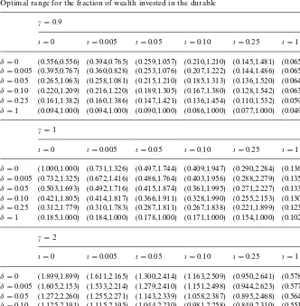
Table 1
Optimal range for the fraction of wealth invested in the durable
c"0.9
n"0 n"0.005 n"0.05 n"0.10 n"0.25 n"1
d"0 (0.556,0.556) (0.394,0.765) (0.259,1.057) (0.210,1.210) (0.145,1.481) (0.065,2.045)
d"0.005 (0.395,0.767) (0.360,0.828) (0.253,1.076) (0.207,1.222) (0.144,1.486) (0.065,2.039)
d"0.05 (0.265,1.063) (0.258,1.081) (0.215,1.210) (0.185,1.313) (0.136,1.520) (0.064,1.984)
d"0.10 (0.220,1.209) (0.216,1.220) (0.189,1.305) (0.167,1.380) (0.128,1.542) (0.063,1.920)
d"0.25 (0.161,1.382) (0.160,1.386) (0.147,1.421) (0.136,1.454) (0.110,1.532) (0.059,1.731)
d"1 (0.094,1.000) (0.094,1.000) (0.090,1.000) (0.086,1.000) (0.077,1.000) (0.049,1.000)
c"1
n"0 n"0.005 n"0.05 n"0.10 n"0.25 n"1
d"0 (1.000,1.000) (0.731,1.326) (0.497,1.744) (0.409,1.947) (0.290,2.284) (0.136,2.901)
d"0.005 (0.732,1.325) (0.672,1.416) (0.486,1.764) (0.403,1.956) (0.288,2.279) (0.135,2.879)
d"0.05 (0.503,1.693) (0.492,1.716) (0.415,1.874) (0.361,1.995) (0.271,2.227) (0.133,2.686)
d"0.10 (0.421,1.805) (0.414,1.817) (0.366,1.911) (0.328,1.990) (0.255,2.153) (0.130,2.497)
d"0.25 (0.312,1.779) (0.310,1.783) (0.287,1.811) (0.267,1.838) (0.221,1.899) (0.123,2.045)
d"1 (0.185,1.000) (0.184,1.000) (0.178,1.000) (0.171,1.000) (0.154,1.000) (0.102,1.000)
c"2
n"0 n"0.005 n"0.05 n"0.10 n"0.25 n"1
d"0 (1.899,1.899) (1.611,2.165) (1.300,2.414) (1.163,2.509) (0.950,2.641) (0.578,2.824)
d"0.005 (1.605,2.153) (1.533,2.214) (1.279,2.410) (1.151,2.498) (0.944,2.623) (0.577,2.800)
d"0.05 (1.272,2.260) (1.255,2.271) (1.143,2.339) (1.058,2.387) (0.895,2.468) (0.564,2.597)
d"0.10 (1.125,2.191) (1.115,2.195) (1.044,2.230) (0.981,2.258) (0.849,2.310) (0.551,2.403)
d"0.25 (0.904,1.888) (0.900,1.889) (0.865,1.897) (0.831,1.905) (0.747,1.922) (0.517,1.959)
d"1 (0.592,1.000) (0.591,1.000) (0.581,1.000) (0.569,1.000) (0.538,1.000) (0.421,1.000) Note: The table shows numerical values of the interval (1/rH1, 1/rH2) for di!erent values of the investor's risk aversion and of the proportional transaction cost rates. The other parameters are set as follows:r"0.01,k"0.069,p"0.22,b"0 ando"0.01.
the percentage transaction costsdandn, while the upper bound appears to be
strictly increasing inn, but not necessarily a monotonic function ofd.13Indeed, it
difn"0 and rH(1, i.e., if
o'(1!c)(r#i/c)#c(r#b).
This is so because we must have 1/rH2"1/rH'1 for d"0 and 1/rH2"1 for d"1. The following proposition con"rms the above analysis.
Proposition 2. Let rH1,rH2 satisfy the conditions of Theorem 3. Then rH1 is strictly increasing innandd,whilerH
2 is strictly decreasing inn.
Proof.It is easy to see from Eqs. (17)}(19) thatrH1"r
1(d,n) andr2H"r2(d,n) for
some continuously di!erentiable functionsr
1,r2. Also, letting
Since t(x) represents the value function for the investor's problem when
K
0"1 and the maximum expected utility is strictly decreasing in the
transac-tion cost ratesdandn(this follows from the fact that the optimal policy always
involves a positive probability of hitting either boundary: see Proposition 4), we must haveLt1(x,r
1(d,n),n)/Ld(0 andLt1(x,r1(d,n),n)n/Ln(0 for allx5r1(d,n)
andLt2(x,r
2(d,n),d)/Ln(0 for alld(x4r2(d,n).
The"rst inequality amounts to
0'Lt1(x,rH1,n) Since the"rst fraction in the above expression is strictly positive (by Proposition 1), we conclude that Lr
1(d,n)/Ld'0. The proof that Lr1(d,n)/Ln'0 and
Lr
2(d,n)/Ln(0 is similar. h
The fact that the upper bound 1/rH2 of the optimal range for the fraction of wealth invested in the durable is not necessarily monotonically increasing in dmay at"rst appear counterintuitive. However, it can be rationalized as follows. An increase in the transaction cost rates d and n a!ects the location of the
optimal range forK/=in two di!erent ways. First, since adjusting the stock of
transaction-avoidance e!ect'). On the other hand, an increase in d or n also induces the
investor to save more to compensate for lower future consumption due to higher future transaction costs: this is obtained by decreasing the upper bound 1/rH2 (and possibly the lower bound 1/rH1) of the optimal range for the fraction of wealth invested in the durable good (the&saving'e!ect). While both e!ects will tend to unambiguously decrease 1/rH1as the transaction cost rates increase, the net impact on 1/rH2depends on which factor dominates.
Since 1/rH1 is decreasing indandnand 1/rH
1"1/rHfor d"n"0, we always
have 1/rH141/rH. On the other hand, since 1/rH2is not necessarily increasing ind, it is possible that 1/rH241/rH, i.e., that the no-transaction region does not contain the Merton line. In this case, the investor always consumes less, for any given level of wealth, than what he would consume in the absence of adjustment costs. The following proposition provides a simple necessary and su$cient condition for this to happen.
Proposition 3. LetrHbe as in Theorem1and letrH2be as in Theorem3.There exists ad3(0,1) such thatrH2'rHif and only ifrH(1,i.e., if and only if
o'(1!c)(r#i/c)#c(r#b).
Proof.The condition onois equivalent to
c[a1m#(1!ca
1)(r#b)]
m (1.
Fixdwith
c[a1m#(1!ca
1)(r#b)]
m (d(1.
Then it follows from Proposition 1 that
rH2'1! 1!d
1!ca
1
'c(r#b)
m "rH.
Conversely, suppose that rH2'rH for some d3(0, 1). Then it follows from Proposition 1 that
0(rH2!rH4c(r#b)(1!d)
m #d!rH
"do!(1!c)(r#i/c)!c(r#b)
m . h
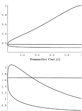
Fig. 1. Boundaries of the optimal range for the fraction of wealth invested in the durable as a function of the transaction cost rate. The graph plots 1/rH1 and 1/rH2againstdfor two di!erent values of the investor's time preference parameter:o"0.01 (top graph) ando"0.10 (bottom graph). The other parameters are set as follows:r"0.01,k"0.069,p"0.22,n"0,b"0.05 andc"1.
a function of the transaction cost ratedfor a log investor (c"1) and for two di!erent values of the time-preference parameter (o"0.01 ando"0.10). In the
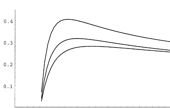
14An optimal policy does not exist in Fig. 2 for
c(cH"J(o!r#i)2#4ri!(o!r#i)
2r "0.815,
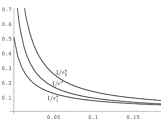
as Assumption 1 is violated in this case. Moreover, ascBcH, the optimal policy involves postponing consumption to increase investment in the stock market. Thus, both boundaries of the no-transaction region converge to zero. In Fig. 3, as bCR, the durable behaves increasingly as a perishable good, so that lim(1/rH1)"lim(1/rH2)"lim(1/rH)"0.
Fig. 2. Boundaries of the optimal range for the fraction of wealth invested in the durable as a function of the investor's relative risk aversion coe$cient. The graph plots 1/r1H, 1/rH2 and 1/rH
against c. The other parameters are set as follows: r"0.01,k"0.069,p"0.22,d"0.05, n"0,b"0.05 ando"0.01.
transaction cost rate is large enough. This re#ects the fact that in the latter case the investor is more impatient and thus initially less willing to save. Since this implies a higher marginal utility for future consumption, a reduction in future consumption due to an increase in transaction costs induces him to increase his savings proportionally more than a less impatient investor. Thus, the&saving'
e!ect dominates the&transaction-avoidance'e!ect.
Fig. 3. Boundaries of the optimal range for the fraction of wealth invested in the durable as a function of the durable's depreciation rate. The graph plots 1/rH1, 1/rH2 and 1/rHagainst b. The other parameters are set as follows:r"0.01,k"0.069,p"0.22, d"0.05,n"0,o"0.01 andc"1.
function of the risk aversion and a monotonically decreasing function of the depreciation rate. Thus, the optimal consumption policy for short-lived durable goods is to purchase small quantities frequently, while the optimal policy for long-lived durables calls for more sporadic and larger purchases. This agrees with the"nding of Hindy and Huang (1993) for the cased"1.
6.2. Stochastic behavior of the investment in the durable
In order to analyze in more detail the stochastic behavior of the investment in the durable, letx
t"=Ht/KHt denote the inverse of the fraction of wealth invested
in the durable at timet. An application of Ito( 's lemma shows that, within the no-transaction region,
dx
t"a(xt) dt#b(xt)Tdwt,
where
a(x)"(r#b)(x!1)#2iu lH(x)
and
Now"xx
0"x3(rH2,rH1), and let
q"infMt50:x
tN(rH2,rH1)N.
denote the time of the next transaction in the durable. Also, let
P
x(q(R)"P(q(RDx0"x)
denote the conditional probability thatqis"nite and let
E
x[q]"E[q Dx0"x]
denote the conditional expectation of q. Finally, "x an arbitrary number
c3(rH2,rH1) and de"ne the scale function
s(x)"
P
xc
exp
A
!2P
yc
a(z)
Db(z)D2dz
B
dyas well as thespeed density
m(x)" 2
s@(x)Db(x)D2.
Proposition 4. If d(1,then P
x(q(R)"1andEx[q](Rfor all x3(rH2,rH1).
Moreover, either boundary of the no-transaction region can be reached with positive probability. On the other hand, if d"1 then P
x(q(R)"1 if
o4r#i#cb and 0(P
x(q(R)(1 otherwise. In either case, the lower
boundary is never reached.
Proof.Sinceu
lH(x)'0 for allx3(rH2,rH1), we have (recalling the standing
assump-tion thati'0)
Db(x)D2'0 ∀x3(rH2,rH1).
Moreover, since botha(x) andb(x) are continuous on (rH2,rH1),
∀x3(rH2,rH1), &e'0 such that
P
x`ex~e
1#Da(x)D
Db(x)D2 dx(R.
Now let
q(x)"
P
xc
(s(x)!s(y))m(y) dy"
P
xc
s@(y)
AP
yc
m(z) dz
B
dy.If d(1, then u
lH(x)'0 for all x3[r2H,rH1], so that s and m are de"ned and
continuous on [rH2,rH1], and we haveq(rH2)(Randq(rH1)(R. The fact that E
in Karatzas and Shreve (1988), while the fact that either boundary can be reached with positive probability follows from Proposition 5.5.22(d).
If d"1, then the above argument is not necessarily true, since u
lH(rH2)"u0(1)"0. On the other hand, since u0(x)"a2(x!1), for anyx'1,
we have in this case
s(x)"
P
xfollows from Proposition 5.5.32(ii) in Karatzas and Shreve (1988), while the fact that the lower boundary is never reached follows from Proposition 5.5.22(c). On the other hand, if o'r#i#cb, then f(1, and hence s(rH1)(R,
s(rH2)"s(1)'!R,q(rH1)(R and q(rH2#)"q(1#)"#R, so that it follows from Propositions 5.5.29 and 5.5.32 in Karatzas and Shreve (1988) that 0(P
x(q(R)(1. The fact that the lower boundary is never reached follows
from the fact that q(#R)"#R and Proposition 5.5.29 in Karatzas and Shreve (1988). h
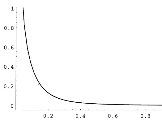
Fig. 4. Steady-state average fraction of wealth invested in the durable as a function of the transaction cost rate. The graph plots the average ofKH/=Hunder the steady-state distribution against d. The other parameters are set as follows: r"0.01,k"0.069,p"0.22, n"0,b"0.05,o"0.01 andc"1.
and that
f(x)" m(x)
:rH1
rH2m(y) dy
is a stationary (or steady-state) probability density (Borodin and Salminen, 1996, Section II.12). In addition,xis ergodic and the distribution ofx
tconverges
to the stationary distribution, that is
lim
t?=
A
sup
A|B
(*rH2,rH1+)
K
P
x(xt3A)!
P
A
f(z) dz
KB
"0where B([rH
2,rH1]) denotes the Borel sigma-"eld on [rH2,rH1] (Borodin and
Salminen, 1996, Section II.35}36).
Fig. 4 shows the steady-state average fraction of wealth invested in the durable as a function of the transaction cost rate d. As it could be expected, even though the no-transaction region is monotonically increasing in this case (as shown in Fig. 2), the steady-state average proportional investment in the durable good declines monotonically as the transaction costs increase.
6.3. Frequency of transactions in the durable
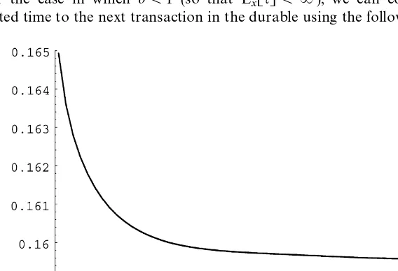
For the case in which d(1 (so that E
x[q](R), we can compute the
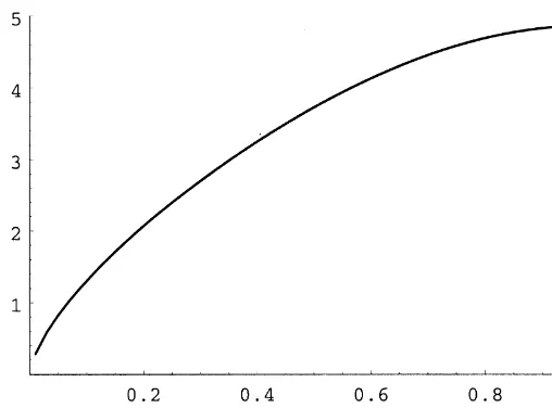
Fig. 5. Expected length of time (in years) to the next transaction in the durable as a function of the fraction of wealth invested in the durable. The graph plotsE
x[q] against 1/x"KH/=Hfor di!erent
values ofd. Each curve is plotted over the optimal range forKH/=H. The other parameters are set as follows:r"0.01,k"0.069,p"0.22,n"0,b"0.05,o"0.01 andc"1.
Proposition 5. Suppose that d(1. Then the function ¹(x)"E
x[q] solves the
ordinary diwerential equation
1
2Db(x)D2¹A(x)#a(x)¹@(x)#1"0
on(rH2,rH1),with boundary conditions¹(rH2)"¹(rH1)"0.
Proof.This follows immediately from Karlin and Taylor (1981, p. 192). h
Fig. 5 plots the expected length of time (in years) to the next adjustment in the stock of the durable¹(x)"E
x[q] as a function of the current fraction of wealth
invested in the durableKH/=H"1/xfor di!erent levels of the transaction cost rate d. While the values in Fig. 5 are conditional expectations based on the current value ofx, Figs. 6 and 7 plot the unconditional expectation of the time to the next transaction in the durable under the steady-state distribution forx, as a function of the transaction cost ratedand of the depreciation rateb. The latter
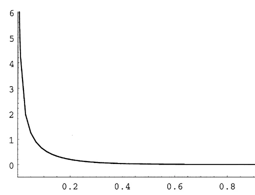
Fig. 6. Steady-state average time to the next transaction in the durable as a function of the transaction cost rate. The graph plots the unconditional mean of the time to the next transaction under the steady-state distribution ofxas a function ofd. The other parameters are set as follows: r"0.01,k"0.069,p"0.22,n"0,b"0.05,o"0.01 andc"1.
case of a divisible durable good than in the case of an indivisible good studied by Grossman and Laroque (1990).
An alternative assessment of the frequency of transactions in the durable can be obtained by examining the expected discounted value of the lifetime pur-chases and sales of the durable.
Proposition 6. Letj,j1,j2be arbitrary constants with
j'r#2irH1#n
crH1 .
Then
E
CP
=0
e~jtD j1dIHt#j
2dDHt D
K
KH0"K,=H0"=D
(Rfor all(=,K) withK'0and=/K3[rH2,rH1]if and only if
E
CP
=0
e~jt(j1dIH
t#j2dDHt)
K
KH0"K, =0H"=D
"Kg(=/K;j,j1,j2),whereg(x)"g(x;j,j1,j2)solves the ordinary diwerential equation
1
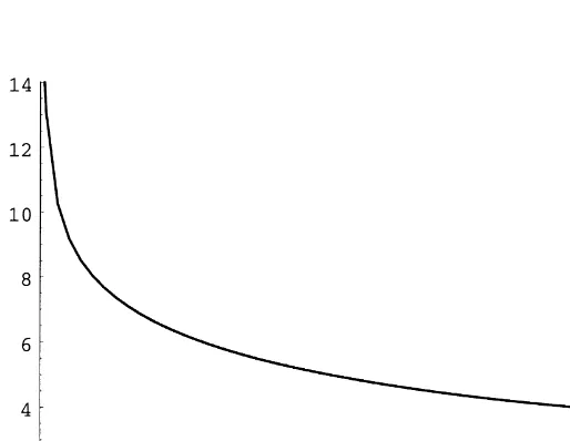
Fig. 7. Steady-state average time to the next transaction in the durable as a function of the depreciation rate. The graph plots the unconditional mean of the time to the next transaction under the steady-state distribution ofxfor di!erent values ofb. The other parameters are set as follows: r"0.01,k"0.069,p"0.22,d"0.05,n"0,o"0.01 andc"1.
on[rH2,rH1]with boundary conditions
g(rH1)!(rH1#n)g@(rH
1)#j1"0
and
g(rH2)!(rH2!d)g@(rH2)!j
2"0.
Proof.Suppose"rst that there is a solutiongto ODE (26) with the associated boundary conditions and let C(=,K)"Kg(=/K). An application of Ito( 's
lemma gives
C(=,K)"e~jtC(=H
t,KHt)!
P
t
0
e~jsC
W(=Hs,KsH)hHsTpdws
!
P
t0
e~js(12C
WW(=Hs,KHs)D hHsTp D2
#C
W(=Hs,KHs)[r=Hs#hHsT(k!r)!(r#b)KHs]
!C
#
P
tin the previous expression has zero expectation, so that
C(=,K)"E
C
e~jt=HLetting n"hH/=Hdenote the portfolio weights process, we will show below
that
is a martingale, so that
E[e~jt=H
t]4E
C
expAP
t
0
(r#nT
s(k!r1)!j) ds
B
NtD
4exp
AA
r#2irH1#ncrH1 !j
B
tB
E[Nt]"exp
AA
r#2irH1#ncrH1 !j
B
tB
=P0 as tPR.
Conversely, letting
C(=,K)"E
CP
=0
e~jt(j1dIHt#j
2dDHt)
K
KH0"K,=H0"=D
,it is easily veri"ed that C is homogeneous of degree one in (=,K), so that
C(=,K)"Kg(=/K) for some function g. The ODE forg then follows from
Ito( 's lemma and the fact that the process
e~jtC(=
t,Kt)#
P
t
0
e~js(j1dIH
s#j2dDHs)
is a martingale. Finally, to show that
u lH(xt)
x
t
4rH1#n
crH1 , let
l(x,y)"b
1log[yx!a1(x!1)]#b2log[yx!a2(x!1)].
Sincelis strictly increasing inyand
rH1#n
crH1 rH2'
rH2!d
c ,
it follows from (17) and (18) that
l
A
rH1,rH1#ncrH1
B
"log(lH)(lA
rH2,rH1#n
crH1
B
. The concavity oflin xthen impliesl
A
x,rH1#ncrH1
B
5log(lH) for all x3[rH2,rH1]. The claim now follows from the fact thatl
A
x,ulH(x)x
B
"log(lH)15The same monotonic pattern prevails in the case in whicho"0.10, even though (as shown in Fig. 1) the boundaries of the no-transaction region are non-monotonic in this case.
Fig. 8. Expected discounted lifetime purchases of the durable over existing stock as a function of the transaction cost rate. The graph plots the unconditional mean ofg(x; 0.10, 1, 0) under the steady-state distribution of x for di!erent values of d. The other parameters are set as follows: r"0.01,k"0.069,p"0.22,n"0,b"0.05,o"0.01 andc"1.
The above proposition allows to compute the expected discounted value of the lifetime purchases (respectively, sales) of the durable good, conditional on the current values of=HandKH, by solving ODE (26) forgwithj
1"1 and
j2"0 (respectively,j1"0 andj2"1). Figs. 8 and 9 report the unconditional expected discounted values of the lifetime purchases and sales of the durable, as a fraction of the initial stock of the durable, for di!erent levels of the transaction cost rated. The unconditional expected discounted values are computed under the steady-state distribution of x and the discount rate j is set at 0.1. While the expected discounted purchases and sales are both monotonically decreasing in d, the latter are more responsive than the former to changes in selling costs.15
6.4. The portfolio policy
Fig. 9. Expected discounted lifetime sales of the durable over existing stock as a function of the transaction cost rate. The graph plots the unconditional mean ofg(x; 0.10, 0, 1) under the steady-state distribution of x for di!erent values of d. The other parameters are set as follows: r"0.01,k"0.069,p"0.22,n"0,b"0.05,o"0.01 andc"1.
transaction costs. However, their risk aversions, and hence the fraction of their wealth invested in stocks, are changed as a result of the presence of transaction costs. More precisely, the following proposition shows that investors are less risk averse than they would be in the absence of transaction costs when their wealth is large relative to the stock of durable (i.e., immediately before or after a purchase), and more risk averse when their wealth is small (i.e., immediately before or after a sale).
Proposition 7. LetrH1,rH2satisfy the conditions of Theorem3.Then C(rH1)4c4C(rH2).
Proof. Let lH be the constant in (17) and (18). Since u
lH(rH1)"(rH1#n)/c and
u
lH(rH2)"(rH2!d)/cby (15), (17) and (18), we have from (16):
C(rH1)" rH1 u
lH(rH1)
" crH1
rH1#n4c4
crH2
rH2!d"
rH2 u
lH(rH2)
"C(rH2). h
16As in Table 1, we setb"0 to allow direct comparison with the values in Table 1 of Grossman and Laroque (1990).
Table 2
Optimal range for the fraction of wealth invested in stocks
c"0.9
n"0 n"0.005 n"0.05 n"0.10 n"0.25 n"1
d"0 (1.354,1.354) (1.354,1.357) (1.354,1.372) (1.354,1.383) (1.354,1.404) (1.354,1.443)
d"0.005 (1.349,1.354) (1.349,1.357) (1.347,1.372) (1.346,1.382) (1.344,1.403) (1.341,1.443)
d"0.05 (1.282,1.354) (1.281,1.356) (1.273,1.369) (1.266,1.379) (1.251,1.400) (1.220,1.441)
d"0.10 (1.191,1.354) (1.189,1.356) (1.178,1.367) (1.167,1.377) (1.146,1.398) (1.094,1.439)
d"0.25 (0.887,1.354) (0.885,1.356) (0.873,1.364) (0.862,1.373) (0.836,1.392) (0.768,1.435)
d"1 (0.000,1.354) (0.000,1.355) (0.000,1.361) (0.000,1.366) (0.000,1.380) (0.000,1.421)
c"1
n"0 n"0.005 n"0.05 n"0.10 n"0.25 n"1
d"0 (1.219,1.219) (1.219,1.223) (1.219,1.249) (1.219,1.269) (1.219,1.307) (1.219,1.384)
d"0.005 (1.211,1.219) (1.210,1.223) (1.208,1.249) (1.207,1.268) (1.205,1.307) (1.201,1.384)
d"0.05 (1.116,1.219) (1.114,1.222) (1.105,1.244) (1.097,1.263) (1.083,1.302) (1.055,1.381)
d"0.10 (0.999,1.219) (0.997,1.222) (0.986,1.241) (0.976,1.259) (0.957,1.297) (0.915,1.378)
d"0.25 (0.677,1.219) (0.676,1.221) (0.667,1.237) (0.659,1.252) (0.640,1.286) (0.596,1.369)
d"1 (0.000,1.219) (0.000,1.220) (0.000,1.230) (0.000,1.240) (0.000,1.266) (0.000,1.343)
c"2
n"0 n"0.005 n"0.05 n"0.10 n"0.25 n"1
d"0 (0.610,0.610) (0.610,0.614) (0.610,0.649) (0.610,0.680) (0.610,0.754) (0.610,0.962)
d"0.005 (0.603,0.610) (0.603,0.614) (0.602,0.648) (0.602,0.680) (0.602,0.753) (0.601,0.961)
d"0.05 (0.541,0.610) (0.540,0.613) (0.538,0.644) (0.537,0.674) (0.534,0.746) (0.530,0.953)
d"0.10 (0.476,0.610) (0.476,0.613) (0.474,0.641) (0.472,0.669) (0.469,0.739) (0.463,0.945)
d"0.25 (0.322,0.610) (0.322,0.612) (0.320,0.636) (0.319,0.660) (0.317,0.723) (0.311,0.924)
d"1 (0.000,0.610) (0.000,0.611) (0.000,0.627) (0.000,0.644) (0.000,0.691) (0.000,0.866) Note: The table shows numerical values of the interval ((k!r)/(C(rH2)p2),(k!r)/(C(rH1)p2)) for di!erent values of the investor's risk aversion and of the proportional transaction cost rates. The other parameters are set as follows:r"0.01,k"0.069,p"0.22,b"0 ando"0.01.
cost rates dand n.16 Transaction costs on the durable good appear to have
Fig. 10. Fraction of wealth invested in stocks as a function of the fraction of wealth invested in the durable. The graph plotshH/=HagainstKH/=Hfor di!erent values ofd. Each curve is plotted over the optimal range for KH/=H. The other parameters are set as follows: r"0.01,k"0.069,
p"0.22,n"0,b"0.05,o"0.01 andc"1.
of transaction costs. This ratio would#uctuate between 1.210 and 1.223 with a transaction cost of 0.5% in either direction, and between 0.640 and 1.286 with a transaction cost of 25%.
Fig. 10 shows, for the logarithmic case (c"1) and for di!erent levels of the transaction cost rates, how the fraction of wealth invested in stocks, hH/=H,
varies as a function of the fraction of wealth invested in the durable,KH/=H.
While the relationship between hH/=H and KH/=H is non-monotonic, an
increase in the transaction cost rates seems to have the unambiguous result of reducing the fraction of wealth invested in stocks, for any given level of the investor's current consumption and wealth within the no-transaction region. The next proposition con"rms that this is indeed the case.
Proposition 8. Let rH1,rH2 satisfy the conditions of Theorem 3 and let x3(rH2,rH1).
ThenC(x)increases asdornincrease,as long asxremains in the no-transaction region.
Proof.Ifx3(rH2,rH1), then
C(x)"!xtA(x)
t@(x)"
x
u lH(x)
wherelHis the constant in (17) and (18). Since it follows immediately from the de"nition thatu
lH(x) is increasing inlH, it is enough to show thatLlH/Ld(0 and
LlH/Ld(0 then follows immediately from Propositions 1 and 2. The proof that LlH/Ln(0 is similar. h
Hence, the optimal portfolio weights are a linearly decreasing function of the fraction of wealth invested in the durable. Alternatively,
hH
so that the optimal portfolio policy involves investing a constant fraction of liquid wealth=H
t!KHt in stocks. Moreover, it can be shown thata2'1/cand
a2P1/c as bPR. Both of these results are consistent with the "ndings of Hindy and Huang (1993), who considered irreversible purchases of the con-sumption good.
Fig. 11 plots the steady-state average fraction of wealth invested in stocks as a function of the transaction costs rated. Even though within the no-transaction region proportional investment in the stock can be higher or lower than in the Merton case, the average proportional investment is monotonically decreasing in the transaction cost rated, and thus always lower than in the Merton case.
6.5. Welfare impact of transaction costs
Fig. 11. Steady-state average fraction of wealth invested in stocks as a function of the transaction cost rate. The graph plots the steady-state average ofhH/=Hagainstd. The other parameters are set as follows:r"0.01,k"0.069,p"0.22,n"0,b"0.05,o"0.01 andc"1.
Fig. 13. Welfare impact of transaction costs. The graph plots the combinations of initial wealth and transaction cost ratedthat would give a logarithmic investor a constant lifetime expected utility. The other parameters are set as follows:r"0.01,k"0.069,p"0.22,b"0.05,n"0,o"0.01 and
c"1.
a corresponding decrease in the expected level of sales (as shown in Fig. 10). In fact, it follows from Proposition 4 that whend"1 the lower boundary of the no-transaction region is never reached, and hence that expected sales and costs equal zero.
7. Conclusions and extensions
We have examined a continuous-time model in which an investor derives utility from the service#ow provided by a durable consumption good. Adjust-ment of the stock of the durable is costly and entails a proportional transaction cost. Our analysis thus complements that of Grossman and Laroque (1990), who considered the case in which adjustment in the stock of durable involves payment of transaction cost proportional to the existing stock (rather than to the amount bought or sold). We show that an optimal consumption policy exists under the same set of conditions that are necessary and su$cient for existence in the absence of transaction costs. Moreover, we provide a closed-form expression for the value function in terms of three constants solving a system of nonlinear equations.
For the case of no-transaction costs, a change of variables reduces this problem to the one studied in Merton (1971). The optimal policies consist of maintaining a constant fraction of wealth invested in the durable and constant portfolio weights. In the presence of transaction costs, the optimal consumption policy consists of maintaining the fraction of total wealth invested in the durable good in a non-stochastic interval, which is easily computed. This interval may or may not include the ratio of durable to wealth that would be optimal in the no-transaction case. The optimal portfolio strategy involves investing in the same portfolio of risky assets that would be optimal in the absence of transac-tion costs, but the fractransac-tion of wealth allocated to risky assets is stochastic and depends on the current level of wealth relative to the stock of durable. Since the fraction of wealth invested in the durable is within a deterministic interval, the same is true for the fraction of wealth invested in stocks. We show that this interval always brackets the proportion that would be optimal in the absence of transaction costs. Moreover, numerical simulation reveals that this interval is typically small, so that the optimal investment strategy is not very sensitive to the presence of transaction costs for adjusting durable consumption. We also provide an explicit solution for the case in which the transaction cost rate for selling the durable is 100%. Clearly, the optimal consumption policy in this case involves never selling the durable.
Since the investor's optimal consumption policy does not satisfy the usual
"rst-order condition due to the presence of transaction costs, the Consump-tion-based Capital Asset Pricing Model (CCAPM) would not hold in equilib-rium in the economy we study. On the other hand, since investors still hold the same portfolio of risky assets (the mean-variance e$cient portfolio) the standard Capital Asset Pricing Model (CAPM) would hold in equilibrium. This is analogous to what Grossman and Laroque (1990) reported for the case of an indivisible durable good.
consump-tion good, as long as the utility funcconsump-tion is additive and the relative price of the two goods is constant. The value function for the extended problem is given by
v(=
0,K0)" max
W10`W20/W0
v
1(=10,K0)#v2(=20),
wherev
1is the value function for the problem with only the durable good (as
studied in this paper) andv
2is the value function for the problem with only the
perishable good (as in Merton, 1971). The optimal consumption and investment policies can also be immediately retrieved. Clearly, the CAPM would still characterize the equilibrium in this economy, while the CCAPM would hold relative to aggregate nondurable consumption, but not relative to aggregate total consumption.
8. For further reading
The following references are also of interest to the reader: CvitanicH and Karatzas, 1996; Harrison, 1985.
Appendix A
Before embarking on the proof of Theorem 2, whose argument is adapted from Davis and Norman (1990), we start with a preliminary result.
Lemma A.1. Under the assumptions of Theorem2,the functionvdexned in(13)is concave and satisxes:
max
h
C
1
2DhTpD2vww#[r(w!k)#hT(k!r1)!bk]vw
!bkv
k!ov#
(ak)1~c
1!c
D
40 (A.1)onS, with equality on NT. Moreover,
nv
w!vk50on S, with equality on B (A.2)
and
dv
w#vk50onS, with equality on S. (A.3)
Proof.Recalling the de"nition ofvand lettingx"w/k, we have
v
and
v
ww(w,k)vkk(w,k)!vwk(w,k)2
"!ck~2(1`c)((1!c)t(x)tA(x)#ct@(x)2)50,
where the"rst inequality follows from the strict concavity oft and the second inequality follows from (11). This establishes the concavity ofv. On the other hand,
nv
This establishes (A.2). The proof of (A.3) is similar, while (A.1) follows immedi-ately from (9) and (10). h
Proof of Theorem 2.Since
hH(w,k)"!(ppT)~1(k!r1) t@(w/k) (w/k)tA(w/k)w
and the functiont@(x)/(xtA(x)) is continuous and hence bounded on [rH2,rH1], we conclude thatDhH(w,k)D4gw holds for someg(Rand all (w,k)3N¹. Also, since the de"nition ofhHimplies thathH(jw,jk)"jhH(w,k) for allj'0,hHis Lipschitz continuous on N¹. The existence and uniqueness of processes (=H,KH,IH,DH) satisfying the conditions of the theorem for all t(q"
infMt50:=H
t"KHt"0Nthen follows from the construction of di!usions with
oblique re#ections in Lions and Sznitman (1984) or Dupuis and Ishii (1993) (see the proof of Lemma 9.3 in Shreve and Soner (1994) for details).
We will start by showing that q"R a.s., so that (IH,DH,hH)3HK (=
0,K0).
Recalling the de"nition ofv, an application of Ito( 's lemma shows that
Since the function (t@)2/(t tA) is continuous, and hence bounded, on [rH2,rH1] and (1!c)tis bounded below away from zero (because of (11)), the above implies that
0(lim
ttq
Dv(=
t,Kt)D(R onMq(RN.
On the other hand, (8) implies that
lim
Thusq"R, almost surely. Next, let
M
An application of Ito( 's lemma shows that
M(t)"v(=
It then follows from Lemma A.1 that the "rst three integrals in the previous expression are identically zero. Turning next to the stochastic integral, we have from the continuity ofxct@(x) that
(I,D,h)3HK (=
0,K0) that the stochastic integral has zero expectation. Therefore,
v(=
where the second equality follows from the monotone convergence theorem and the third from (A.4), using the fact that 1/[(1!c)t] is bounded below away from
zero onN¹and that the processNin (A.5) is a martingale. Therefore,vis indeed the lifetime expected utility from following the proposed optimal policy.
To conclude the proof, we only need to show that
v(=
Suppose at "rst that c(1. It then follows easily from the de"nitions that there exists a constantge'0 such that
Dv(w,k)D#Dwv
It then follows from the generalized Ito( 's lemma that
#
P
tit follows from Lemma A.1 and the fact thatv
w'0 that the"rst three integrals
in the above expression are nonpositive, while the term in the summation is nonpositive by the concavity of ve. We then conclude from (A.9) that Me is a supermartingale. Hence,
SinceveBvaseB0, we obtain the desired inequality.
Finally, suppose thatc'1. Fix an arbitraryjwith 0(j(r/(r#(1#n)b)
and for anye'0 let ve(w,k)"v(w#e,k#je). It can be immediately veri"ed from the de"nitions thatveandve
ware bounded onS. Moreover,
12DhTpD2ve
ve(=
where the last equality follows from the boundedness ofve. SincevePvaseB0, we conclude that the policy (IH,DH,hH) is optimal for allcO1. h
Proof of Lemma 1.It is easy to verify that any solution of the ODE (14) satis"es
Dul(x)!a
1(x!1)Db1Dul(x)!a2(x!1)Db2"l
for someland that any nonnegative solution has one of three possible shapes on the positive orthant:
(see Lemma 3 in Grossman and Laroque (1987) for details). We can rule out the
"rst two solutions as follows. Let
f(x)"t@(x)2 all x. This rules out the "rst two solutions. Thus, u
l(x)5max[a1(x!1),
a2(x!1)]. h
Proof of Proposition 1.Let
which are de"ned for x3[r
(A.16), this implies that, for any givenr
23[r2,r62], the equationl1(r1)"l2(r2) has
two di!erent solutions: the "rst with r
1(min[r(1,r2], and the second with
r
1'max[r(1,r2]. Since by assumptionrH1'rH2, we must also haverH1'r(1. The
latter inequality impliesg'0.
Finally, lettingfbe the function in (A.12), (20) and the continuity oftimply thatf(rH2)"f(rH1)"0. Sinceu
Moreover, (15) and (18) imply
ulH(rH2)"(rH2!d)/c.
Thus,
(o!r!cb#i)(rH2!d)#c(r#b)(rH2!1) i/c(rH2!d) 41. Rearranging the latter inequality givesrH24r(
![Fig. 5 plots the expected length of time (in years) to the next adjustment in thestock of the durable" ¹(x)"E�[�] as a function of the current fraction of wealthinvested in the durable KH/=H"1/x for di!erent levels of the transaction costrate �](https://thumb-ap.123doks.com/thumbv2/123dok/3104371.1376515/28.468.69.334.331.529/expected-adjustment-thestock-function-fraction-wealthinvested-transaction-costrate.webp)