isprs archives XLI B5 857 2016

AUTOMATIC WATERLINE EXTRACTION FROM SMARTPHONE IMAGES

M. Kröhnert

Institute of Photogrammetry and Remote Sensing, Technische Universität Dresden, Germany Melanie.Kroehnert@tu-dresden.de

Commission V, WG V/5

KEY WORDS: Flood monitoring, Crowdsourcing, Smartphones, Image analysis, Texture measures

ABSTRACT:

Considering worldwide increasing and devastating flood events, the issue of flood defence and prediction becomes more and more important. Conventional methods for the observation of water levels, for instance gauging stations, provide reliable information. However, they are rather cost-expensive in purchase, installation and maintenance and hence mostly limited for monitoring large streams only. Thus, small rivers with noticeable increasing flood hazard risks are often neglected.

State-of-the-art smartphones with powerful camera systems may act as affordable, mobile measuring instruments. Reliable and effective image processing methods may allow the use of smartphone-taken images for mobile shoreline detection and thus for water level monitoring. The paper focuses on automatic methods for the determination of waterlines by spatio-temporal texture measures. Besides the considerable challenge of dealing with a wide range of smartphone cameras providing different hardware components, resolution, image quality and programming interfaces, there are several limits in mobile device processing power. For test purposes, an urban river in Dresden, Saxony was observed. The results show the potential of deriving the waterline with subpixel accuracy by a column-by-column four-parameter logistic regression and polynomial spline modelling. After a transformation into object space via suitable landmarks (which is not addressed in this paper), this corresponds to an accuracy in the order of a few centimetres when processing mobile device images taken from small rivers at typical distances.

1. INTRODUCTION

Since the last prominent flood event in Dresden, Germany, in year 2013, the issue of precise and wide-spread water level monitoring became strongly increasing importance. In this context, a privately organised flood event map, hosted on Google Maps, gained worldwide attention. The map shows several information about flood-affected regions, e.g. in terms of focal points for provision and donation as well as blocked public roads. Everyone could update the map with rational information, whereby cartographic top actualities up to a few minutes could be achieved. The crowdsourcing concept became acquainted as it was effective in supporting the organisation of volunteer hands. Further developing this issue, gauging systems that offer accurate but spatially sparse information about water levels of significant water bodies should be densified by crowdsourced water level information in case of flood events.

Because of its history in flood events, an urban riverside, situated in Dresden, was chosen for study purposes (see section 2.1). On the hardware side, smartphones with inbuilt high-resolution cameras, orientation components based on GNSS and Micro-Electro-Mechanical Systems (MEMS) as well as powerful processing units may act as photogrammetric measurement instruments. Section 2.2 provides a detailed view of the employed device.

Section 3 presents the methodical workflow and its single issues for flowing waterline detection using smartphone-taken images in terms of on-device-processing. Besides, it takes account of pre-processing steps for data preparation as well as post-processing for visualisation purposes. Finally, section 4 and 5 discuss the quality of the derived waterline, assess computational costs, describe approaches for appropriate enhancements and give an outlook for prospective works towards water level determination by image-to-model intersection.

2. DATA ACQUISITION

The chapter of data acquisition comprises the presentation of an urban study area as well as the measuring device which is a standard smartphone with inbuilt camera and orientation units. Section 2.3 describes the way of input data acquisition by image sequences.

2.1 Study region

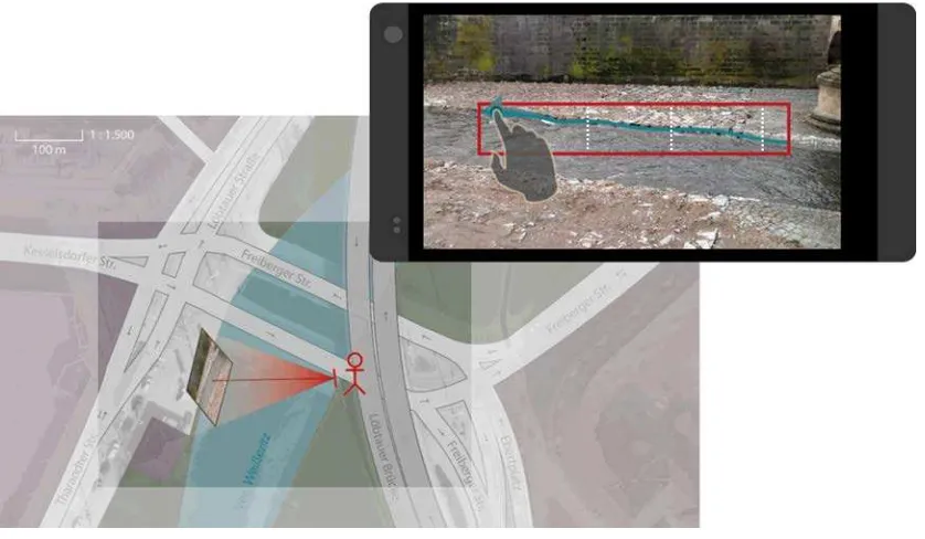
The study region is the urban river Weißeritz in Dresden. The viewpoint for image capturing was located next to an important junction, business park and residential area (Figure 1), where the riverbanks are siliceous and thus the shorelines do not follow distinct edges. Unfortunately, despite its essential location and its flooding potential, the river is so far ungauged.

2.2 Measuring device

For the purpose of crowdsourcing-based data acquisition for densifying water level monitoring and hence to deal with the central issue of waterline detection, consideration should be given to use a widely spread measurement instrument which can acquire, process and share data. Smartphones with their inbuilt cameras, orientation units and intense processing power solve these issues. Todays global smartphone subscription amounts to 3.4 million with rising trends (Ericsson, 2015) and thus, smartphones seem to be the best solution serving the purpose of well-suited ubiquitous measurement devices.

For the experimental research, the Android smartphone HTC One M7, bought out in 2013, equipped with a camera and a Snapdragon 600, 1.7 GHz quad-core processor, acted as measuring device (see Table 1 for closer camera specifications).

Sensor type 1/3’ BackSide Illumination (BSI) sensor, crop factor: 7.21

Resolution Photo: 4.0 MPx, Video: 2.1 MPx Pixel size 2.0 µm

Lens 3.8 mm (effective focal length: 28 mm)

Table 1: HTC One M7, Camera specifications

2.3 Image sequences

Considering the general behaviour of flowing water and thus the behaviour of its shoreline, it becomes obvious that one unique waterline cannot exist due to motion events within the nearshore environment, e.g. unregular waves that will never touch the riverbank similarly. Consequently, the use of single image analysis for the shoreline determination considering flowing water seems to be not very useful (Figure 2). Furthermore, image sequences offer a considerable base for image segmentation using temporal textures due to the variability of the flowing water surface appearance caused by water wave reflections.

Previous works of Koschitzki (2015), Koschitzki et al. (2014) and Mulsow et al. (2014) used single cameras, mounted on tripods for monitoring water levels by image sequences and in succession applied image sequence analyses for the observation of lentic water areas. An approach for waterline detection in case of flowing waters based on spatial texture analyses has been presented in Kröhnert et al. (2015).

Figure 2: Variability of flowing river shorelines in detail: Image frames 01, 13 & 25 of short-time image sequence

(from left to right)

Due to the concept of waterline detection by expanding the image analysis to the timeline and thus determining spatio- temporal textures, the acquisition of short image sequences (typically a few seconds) is a prerequisite (Garg et al., 2004 & Szummer et al., 1996). However, the use of sophisticated camera setups conflicts with the idea of on the fly level detection with the aid of the public and because of that, it has to be thought about mobile multi-image recording strategies. Thereby, an important difference between the application of stationary cameras and hand-held smartphone cameras referring to the computational and internal store capacities limits has to be considered. While the task of photo cameras focusses on the acquisition of images only, smartphones have to manage various background tasks and thus they have to share their processing and storing power with several applications that reveals limitations referring to the continuous shooting of high-resolution images. In case of Figure 1: Study region of river Weißeritz and nearshore environment situated in Dresden (left);

smartphones with minor computational power, the human operator has to wait up to a second between two consequent images, which is quite unsuitable for image sequences exceeding five images. On this account, the use of short-time image sequences may restrict the spatial resolution due to image compression but otherwise, it leads to a high improvement in matters of the temporal resolution.

Considering the present approach, the mandatory need of information about the temporal behaviour is obvious. Due to short recording distances, image compressions allowing for the waterline mapping using image data derived from image sequences with high temporal resolution becomes acceptable. For the detection of shorelines from urban flowing waters, the most helpful, empirically determined rate for short image sequence recording amounts to 5 frames per second (fps) over 5 seconds. These attributes are highly correlated with the significance of pixels temporal variability which also holds good for slow flowing waters as well as the duration of data acquisition and processing. In addition, the algorithm makes use of the highest available device-dependent video resolution (e.g. 1080 p/ 2.1 MPx, see Table 1).

3. DATA PROCESSING METHODS

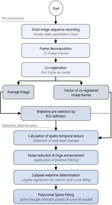
The workflow for waterline derivation (Figure 3) consists of two main steps: First, the recorded image sequence has to be separated into single frames in preparation for their co-registration (section 3.1.1). Because of limited memory and processing power, it makes no sense to analyse the full frames for the waterline. After an initial user-supported rough waterline selection, a Region Of Interest (ROI) will be specified (section 3.1.2). Further investigations comprise in core the calculation of spatio-temporal texture data (section 3.2.1) followed by a bilateral filter approach for spatio-temporal noise reduction (section 3.2.2). Afterwards, a column-by-column curve fitting method based on the four-parameter logistic regression that comprises the present grey values will be executed. In sum, the estimated inflection points represent the waterline with subpixel potential (section 3.2.3). For shoreline refinement, a polynomial spline fit through all determined edge points leads to a continuous waterline representation.

3.1 Pre-Processing

Regarding the record of short image sequences, the present approach has to deal with the problem of a slightly moving hand-held camera. Unfortunately, this juddering is highly correlated with the subsequent spatio-temporal texture analysis. Neglecting would lead to an erroneous detection because of distorted pixel pairs within the image sequence.

3.1.1 Frame decomposition and Co-Registration

To address this concern, the image sequence has to be decomposed to its single frames, followed by their co-registration. The first image usually acts as master scene to which all following frames will be co-registered. The described method acts in a sequential way until all images are registered in relation to the master image.

The Android implementation utilises libraries of the well-established OpenCV4Android SDK library, version 3.0.0 (based on Bradski, 2000).

Firstly, keypoints and their consequent descriptors are computed respectively for master and slave images using the Oriented Features from Accelerated Segment Test (FAST) and the Rotated Binary Robust Independent Elementary Features (BRIEF) algorithm (ORB, Rublee et al., 2011) which includes FAST´s keypoint detector and BRIEF´s descriptor extractor. The implementation of ORB instead of the prevalent Scale-Invariant Feature Transform (SIFT) or Speeded Up Robust Features (SURF) algorithms is motivated by its licence policy. Whereas SIFT and SURF are patented, ORB is a fast alternative that is minimally restricted by Berkeley´s Software Distribution (BSD). Afterwards, a brute force descriptor matching assigns the closest descriptor of the slave data to each descriptor of the master dataset. These matches will be introduced as query (or learning) data due to the master and training point data referring to the slave, to estimate the prevailing valid homography. In order to obtain reasonable results, the appropriate reprojection error must be minimised. Regarding the model computation, the occurrence of non-fitting points due to the train and query point dataset cannot be neglected. Thus, an iterative RANdomSAmple Consensus (RANSAC) is applied for model stabilisation whereby the maximum permissible reprojection error for point pair approval is set to 10 Px in order to avoid a too early rejection of separated frames due to some mismatching points, for instance

Frame decomposition

25 Image Frames

Short image sequence recording

Invoke video application (5sec)

Co-registration

Vector of co-registered image frames

Waterline pre-selection by ROI definition

Waterline determination

Calculation of spatio-temporal texture

Detection of grey level changes

Noise reduction & Edge enhancement

Application of bilateral filtering

Polynomial Spline Fitting

Spline though inflection points of curve-fit models

Subpixel waterline determination

Logistic regression for column wise curve fitting

caused by lens distortion. Remaining errors will be reduced during a final Levenberg-Marquardt refinement that improves the reprojection error significantly and converges even if the input is wide of the result. Using the computed homography, the regarded slave image will be warped perspectively. Subsequent to the image sequence co-registration, an average image, comprising all registered frames, will be computed for visualisation purposes (Figure 4).

3.1.2 ROI definition

For simplification of the waterline detection, an initial waterline defining a bounding box around the touched line has to be drawn by the user. Such a minimal interaction will usually be acceptable in a crowdsourcing approach. For this purpose, the previously calculated average image is displayed to the user who has to point along the visible waterline (Figure 1). All in this way selected points define the mentioned bounding box to crop the co-registered images. Due to small display sizes and jittering hands, the bounding box height will be expanded by 20 Px to define the final ROI (see calculated red box in Figure 1).

3.2 Shoreline determination

After cropping all co-registered images, the core element of the waterline detection will be invoked. As already mentioned, the approach is based on spatio-temporal texture analysis followed by a temporal signal noise reduction. Building on this, an approximation of the waterline with subpixel accuracy is calculated for each column with the aid of logistic regression curve modelling and horizontal polynomial spline fitting.

3.2.1 Spatio-temporal texture analysis

In the same way like the sequential image co-registration, the spatio-temporal texture analysis refers to consecutive image pairs (eq. 1). The image matrices � are checked pairwise in succession for absolute grey level differences among corresponding pixels by ����,�− �(�+1)_�,�� which obviously should represent the same

image content due to their co-registration and their short acquisition interval. Changes inside the grey levels point to dynamic image content such as flowing water. They are registered in terms of their magnitude. Moreover, in case of prevailing grey level differences inside the next comparison, the previously determined magnitudes �_�(�,�) will be added pixel-by-pixel to the current results.

��(�,�) = � � ����,�− �(�+1)�,��

�,� �

�=1

(1)

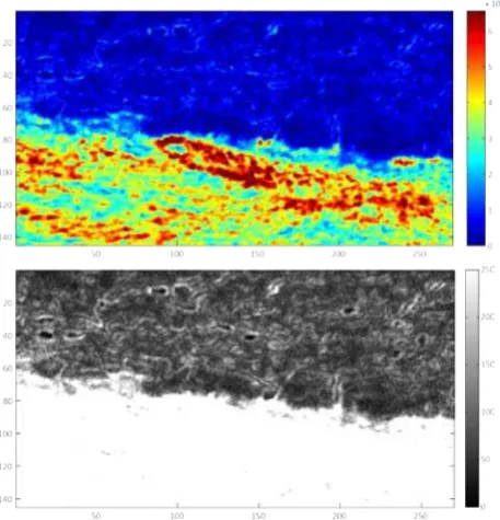
Consequently, the result represents an image matrix summing up the total magnitude of imaged dynamic behaviour (Figure 5-1). Afterwards, an empirically determined threshold separating static from dynamic image content (Figure 5-2) will subdivide the dataset. It should be noted that occasional changes can also result from illumination variations through moving clouds or remaining reprojection uncertainties concerning the co-registration procedure and both could lead to spatio-temporal image noise (section 3.2.2).

3.2.2 Noise reduction and edge enhancement

As already mentioned, the occurrence of temporal noise inside the texture image is not improbable. Common image filtering approaches (e.g. Laplacian of Gaussian) remove image noise reliable but, unfortunately, lead to blurred edges. The problem can be avoided by the application of an edge-preserving smoothing approach such as the bilateral filter which "combines grey levels […] based on both their geometric closeness and their photometric similarity, and prefers near values to distant values in both domain and range” (Tomasi & Manduchi, 1998).

Due to escalation of processing power in relation to filter size, a small neighbourhood around each pixel is advisable for processing on smartphones. In addition to this, two Gaussian filter kernels will be defined by their standard deviation for weighting the pixels depending on their intensity values (range Gaussian σr set to 120 grey levels) and spatial distance (spatial Gaussian, σs, defined by a 5 x 5 Px neighbourhood) which is further explained in Paris et al. (2009). High values of sigma lead to wide areas of similar pixels by preserving large edges like waterlines. Figure 6 shows the textural image before and after the application of bilateral filtering.

Whereas the waterline seems to be almost unaffected, the speckle nearshore and flowing water environment is strongly smoothed even in shadowed and wavy regions.

Figure 4: First frame of image sequence (left), Average image after sequential image co-registration (right)

Figure 5-1: Magnitude of grey level differences before (top); 5-2: After pre-segmentation of spatio-temporal change

3.2.3 Subpixel waterline detection

For image separation and thus for the final shoreline estimation, an edge estimation with subpixel potential will be performed. For this purpose, a four-parameter logistic regression, proposed in Rodbard & McClean (1977), will be applied for each column within the ROI of the filtered spatio-temporal texture image. Thereby, the curve´s inflection point, where the curve changes its direction from concave to convex or vice versa, describes the point for separation of flowing water and shore area. Rodbard´s four-parameter regression is defined by

�(�) =�+ � − �

1 +��

�� �

(2)

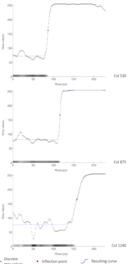
where C describes the mentioned inflection point that matches by horizontal pixel intersection after convergence and thus, represents the limiting point with subpixel precision in its row for each column. Figure 7 visualises the curve modelling for three image columns and marks their estimated inflection points (for better assessment, see Figure 1). It becomes obvious that remained speckle inside the flowing water and nearshore environment cropped out as outliers; however, they will be rejected thanks to the iterative model fit.

3.3 Polynomial Spline Fitting

For data densification and visualisation purposes, it is advisable to apply a polynomial spline estimation using the calculated shoreline points and their corresponding columns as observables. The spline consists of n cubic polynomials in subintervals which

are defined by (n+1) knots regarding the amount of rows. Thus, if the ROI consists of e.g. 300 rows or knots, this would lead to 299 cubic polynoms which define the final polynomial spline and so the continuous waterline approximation (Figure 8). The implementation refers to Apache Commons Math Developers (2016) based on Burden & Faires (1989).

4. RESULTS

In summary it can be said that the proposed method describes an effective method for the determination of flowing water shorelines by analysing spatio-temporal grey value variability and thus shows a useful approach for the distinction of water- and Figure 6: Detail view of wavy and shadowed areas:

Single frame, spatio-temporal texture before and after bilateral filtering (left to right)

Col 1240 Col 875 Col 530

Discrete

grey values Inflection point Resulting curve

Figure 7: Exemplary column-by-column four-parameter logistic regression curve fit for col 530, 875 and 1240

(referring to dashed lines of Figure 1)

shoreland in mobile device imagery. Due to the application of a spatio-temporal texture analysis, shadows and reflexions that appear different within an observation period because of dynamic objects, have only marginal effects to the waterline detection. Additionally, textural outliers (e.g. noise as a consequence of residual reprojection errors due to the co-registration process or radiometric changes within the image sequence which may occur from slight illumination variations caused by moving clouds, could be reduced. For this purpose, the combined application of an edge-preservative bilateral filtering and a column-by-column four-parameter logistic regression that determines the points along the waterline in subpixel range is useful.

However, referring to the proposed texture analysis it should be noted that the technique is currently limited to waterlines appearing almost horizontal within the image data. The current method meets problems in case of an acquisition direction parallel to river´s shoreline and thus its vertical image representation.

Obviously, the computational efforts should always be kept in mind even if the application should work for legacy hardware as well, which is quite important by considering the prospective crowdsourcing concept. Both, Figure 9 and Table 2, show the computation times in relation to the ROI size for the individual processing steps, with a fixed height set to 230 pixels. While the core steps of spatio-temporal texture analysis fulfil realistic crowdsourcing time budget requirements, further work has to be invested to accelerate the steps of image sequence co-registration and logistic regression.

Figure 9: Relationship of the single processing steps and their corresponding computation times in [s] in matters of image size.

Width [Px] (size)

Proc. Step

400 (S) 1000 (M) 1600 (L)

1) Image sequence

decomposition 22.35 22.47 21.81

2) Frame

co-registration 63.66 61.02 60.52

3) Spatio-temporal

texture analysis 0.51 1.18 2.03

4) Noise reduction

(bilateral filtering) 0.31 0.58 0.92

5) 4PL regression 38.73 108.43 198.59

6) Poly. spline fit 0.07 0.17 0.31

� 125.63 193.85 284.18

Table 2: Processing times relating to image size in [s]

Actually, the first steps of frame decomposition and co-registration that go for the whole image should provide equal processing times, but there are numerous reasons for slight derivations, e.g. active background tasks that belong to Android system software, still working activities of other applications due to Android´s life circle (Google, 2016) or even battery status. The current implementation of image co-registration may be to abundant due to the prevalent method of data acquisition. During 3 seconds, the user´s position and orientation might be kept sufficiently constant and thus image adjustment routines (e.g. affine transformations) which consider image translation and rotation only, may be sufficient. Moreover, the geometric transformation between two frames by the enhanced correlation coefficient as a performance criterion for image alignment (published in Evangelidis & Psarakis, 2008), should be taken in consideration for improved performance.

Obviously, shortcomings in view of processing power occur in terms of the image-to-image registration and curve fitting procedures. Appling multi-threading approaches in general and a limitation of the single point arrays to regions closer to the straight shore area in terms of the curve fitting will considerably reduce the computational effort. Furthermore, state-of-the-art smartphones usually offer the possibility to include the graphical processing unit (GPU) that relieves the internal memory as well.

5. FUTURE WORK

As a prospect for the future, the approach should be enhanced for direction-independent waterline derivations. Additionally, the estimated threshold for the definition of dynamic behaviour needs further investigations. An image quantisation of the floating point texture data by clustering due to its contribution could supersede the empirical assessment. Further improvements might be achieved for noise reduction whose results are of quasi-binary nature. Thanks to this, an image labelling (as proposed in Kröhnert et al., 2015) which would be done in preparation for the curve fit could be used to revise the distribution of observed static and dynamic objects in the spatio-temporal domain that could be used further to select a well-fitting regression model. In this way, not only the orientation-dependent applicability issue is solved, but also indentations of the flowing water body could be better detected.

In view of the future and despite source code optimisations it should be noticed, that the intended water level determination by image-to-model intersection needs only a few points (minimum even one) along the waterline and thus the derivation of large waterlines (like image size L in Table 2) and its computational efforts will not be an issue anymore. By translating the waterline points from image into object space, a level determination with accuracies up to a few centimetres seems to be quite possible and marks the next key development.

6. ACKNOLODGEMENT

Gratefully, I acknowledge the European Social Fund (ESF) and the Free State of Saxony for their financial support on a grant.

7. REFERENCES

Apache Commons Math Developers, 2016. The Apache Software Foundation “Commons Math”, Forest Hill, MD, USA

Bradski, G., 2000. The OpenCV Library. Dr. Dobb’s Journal of

Software Tools, 25(11), pp. 120-126.

Burden, R. L. & Faires, J. D., 1989. Numerical Analysis. PWS-Kent, Boston, MA, USA, pp. 126-131.

Ericsson, 2015. “Ericsson Mobility Report - November 2015”, Stockholm, Sweden http://www.ericsson.com/res/docs/2015/ mobility-report/ericsson-mobility-report-nov-2015.pdf

(11 Feb. 2016).

Evangelidis, G. D. & Psarakis, E. Z., 2008. Parametric image alignment using enhanced correlation coefficient maximization. IEEE Transactions on Pattern Analysis and

Machine Intelligence, 30(10), pp. 1858-1865.

Garg, K., & Nayar, S. K., 2004. Detection and removal of rain from videos. In: Proceedings of the IEEE Computer Society

Conference: Computer Vision and Pattern Recognition, 2004. (CVPR 2004), 1, pp. I-528.

Google, 2016. Android Developers “Activity”, Mountain View, CA, USA https://developer.android.com/reference/android/app/ Activity.html (20 Feb. 2016).

Koschitzki, R., 2015. Report on the World Multidisciplinary Earth Sciences Symposium (WMESS) “Monoscopic image sequence analysis for monitoring glacier lake outburst floods”, Prague, Czech Republic (07-11 Sept. 2015).

Koschitzki, R., Schwalbe, E., & Maas, H.-G., 2014. An autonomous image based approach for detecting glacial lake outburst floods. ISPRS - International Archives of the

Photogrammetry, Remote Sensing and Spatial Information Sciences, (XL)5, pp. 376-342.

Kröhnert, M., Koschitzki, R., Maas, H-G., 2015. Report on the 35. Wissenschaftlich-Technische Jahrestagung der DGPF e.V. und Workshop on Laser Scanning Applications: „Wasserlinienextraktion aus optischen Nachbereichsaufnahmen mittels Texturmessverfahren“, DGPF Tagungsband 24/2015, Köln, Germany (16-18 Mar. 2015).

Mulsow, C., Koschitzki, R., Maas, H.-G., 2014. Photogrammetric monitoring of glacier margin lakes. Geomatics,

Natural Hazards and Risk, (6)5-7, pp. 600-613.

Paris, S., Kornprobst, P., Tumblin, J., & Durand, F., 2008. Bilateral filtering: Theory and Applications. Foundation

and Trends in Computer Graphics and Vision, 4(1), pp. 1-73.

Rodbard, D., & McClean, S. W., 1977. Automated computer analysis for enzyme-multiplied immunological techniques. Clinical chemistry, 23(1), pp. 112-115.

Rublee, E., Rabaud, V., Konolige, K., & Bradski, G., 2011. ORB: an efficient alternative to SIFT or SURF. In: Proceedings of the

IEEE International Conference of Computer Vision (ICCV), 2011, pp. 2564-2571.

Szummer, M., & Picard, R. W., 1996. Temporal texture modeling. In: Proceedings of the IEEE International Conference

of Image Processing, 1996, 3, pp. 823-826.