and the Labor Market Impact
of Immigration
George J. Borjas
a b s t r a c t
This paper presents a theoretical and empirical study of how immigration influences the joint determination of the wage structure and internal migra-tion behavior for native-born workers in local labor markets. Using data from the 1960–2000 decennial censuses, the study shows that immigration is associated with lower in-migration rates, higher out-migration rates, and a decline in the growth rate of the native workforce. The native migration response attenuates the measured impact of immigration on wages in a local labor market by 40 to 60 percent, depending on whether the labor market is defined at the state or metropolitan area level.
I. Introduction
Immigrants in the United States cluster in a small number of geo-graphic areas. In 2000, for example, 69.2 percent of working-age immigrants resided in six states (California, New York, Texas, Florida, Illinois, and New Jersey), but only 33.7 percent of natives lived in those states. Similarly, 38.4 percent of immigrants lived in four metropolitan areas (New York, Los Angeles, Chicago, and San Francisco), but only 12.2 percent of natives lived in the four metropolitan areas with the largest native-born populations (New York, Chicago, Los Angeles, and Philadelphia).
Economic theory suggests that immigration into a closedlabor market affects the wage structure in that market by lowering the wage of competing workers and raising the wage of complements. Most of the empirical studies in the literature exploit the geographic clustering of immigrants to measure the labor market impact of
immigra-George J. Borjas is the Robert W. Scrivner Professor of Economics and Social Policy at the Kennedy School of Government, Harvard University; and a Research Associate at the National Bureau of Economic Research. The author thanks two anonymous referees, Alberto Abadie, Richard Freeman, Edward Glaeser, Daniel Hamermesh, Lawrence Katz, Robert Rowthorn, and Stephen Trejo for very helpful comments on an earlier draft, and the Smith-Richardson Foundation for research support. The data used in this article can be obtained beginning October 2006 through September 2009 from the author (gborjas@harvard.edu). [Submitted March 2005; accepted August 2005]
ISSN 022-166X E-ISSN 1548-8004 © 2006 by the Board of Regents of the University of Wisconsin System
tion by defining the labor market along a geographic dimension—such as a state or a metropolitan area. Beginning with Grossman (1982), the typical study relates a meas-ure of native economic outcomes in the locality (or the change in that outcome) to the relative quantity of immigrants in that locality (or the change in the relative number).1 The regression coefficient, or “spatial correlation,” is then interpreted as the impact of immigration on the native wage structure.
There are two well-known problems with this approach. First, immigrants may not be randomly distributed across labor markets. If immigrants tend to cluster in areas with thriving economies, there would be a spurious positive correlation between immigration and wages either in the cross-section or in the time-series. This spurious correlation could attenuate or reverse whatever measurable negative effects immi-grants might have had on the wage of competing native workers.2
Second, natives may respond to the entry of immigrants into a local labor market by moving their labor or capital to other localities until native wages and returns to capital are again equalized across areas. An interregion comparison of the wage of native workers might show little or no difference because the effects of immigration are diffused throughout the national economy, and not because immigration had no economic effects.
In view of these potential problems, it is not too surprising that the empirical liter-ature has produced a confusing array of results. The measured impact of immigration on the wage of native workers in local labor markets fluctuates widely from study to study, but seems to cluster around zero. In recent work (Borjas 2003), I show that by defining the labor market at the national level—which more closely approximates the theoretical counterpart of a closed labor market—the measured wage impact of immi-gration becomes much larger. By examining the evolution of wages in the 1960–2000 period within narrow skill groups (defined in terms of schooling and labor market experience), I concluded that a 10 percent immigrant-induced increase in the number of workers in a particular skill group reduces the wage of that group by 3 to 4 percent. In this paper, I explore the disparate findings implied by the two approaches by focusing on a particular adjustment mechanism that native workers may use to avoid the adverse impacts of immigration on local labor markets: internal migration. A number of studies already examine if native migration decisions respond to immigra-tion. As with the wage-impact literature, these studies offer a cornucopia of strikingly different findings, with some studies finding strong effects (Filer 1992; Frey 1995), and other studies reporting little connection (Card 2001; Kritz and Gurak 2001).3
This paper can be viewed as an attempt to reconcile two related, but so far uncon-nected, strands in the immigration literature. I present a theoretical framework that jointly models wage determination in local labor markets and the native migration
1. See also Altonji and Card (1991), Borjas (1987), Card (1990, 2001), LaLonde and Topel (1991), and Schoeni (1997). Friedberg and Hunt (1995) survey the literature.
2. Borjas (2001) argues that income-maximizing immigrants would want to cluster in high-wage regions, helping to move the labor market toward a long-run equilibrium. The evidence indeed suggests that, within education groups, new immigrants tend to locate in those states that offer the highest rate of return for their skills.
decision. The theory yields estimable equations that explicitly link the parameters measuring the wage impact of immigration at the national level, the spatial correla-tion between wages and immigracorrela-tion in local labor markets, and the native migracorrela-tion response. The model clearly shows that the larger the native migration response, the greater will be the difference between the estimates of the national wage effect and the spatial correlation. The model also implies that it is possible to use the spatial cor-relations to calculate the “true” national impact of immigration as long as one has information on the migration response of native workers.
I use data drawn from all the Census cross-sections between 1960 and 2000 to esti-mate the key parameters of the model. The data indicate that the measured wage impact of immigration depends intimately on the geographic definition of the labor market, and is larger as one expands the size of the market—from the metropolitan area, to the state, to the Census division, and ultimately to the nation. In contrast, although the measured impact of immigration on native migration rates also depends on the geographic definition of the labor market, these effects become smaller as one expands the size of the market. These mirror-image patterns suggest that the wage effects of immigration on local labor markets are more attenuated the easier that natives find it to “vote with their feet.” In fact, the native migration response can account for between 40 to 60 percent of the difference in the measured wage impact of immigration between the national and local labor market levels, depending on whether the local labor market is defined by a state or by a metropolitan area.
II. Theory
I use a simple model of the joint determination of the regional wage structure and the internal migration decision of native workers to show the types of parameters that spatial correlations identify, and to determine if these parameters can be used to measure the national labor market impact of immigration.4Suppose that the labor demand function for workers in skill group iresiding in geographic area jat time tcan be written as:
(1) wijt= XijtLijtη,
where wijtis the wage of workers in cell (i, j, t); Xijtis a demand shifter; Lijtgives the total
number of workers (both immigrants, Mijt, and natives, Nijt); and ηis the factor price
elasticity (with η< 0). It is convenient to interpret the elasticity ηas the “true” impact that an immigrant influx would have in a closed labor market in the short run, a labor market where neither capital nor native-born labor responds to the increased supply.
Suppose the demand shifter is both time-invariant and region-invariant (Xijt= Xi).
This simplification implies that wages for skill group i differ across regions only
because the stock of workers is not evenly distributed geographically.5I assume that the total number of native workers in a particular skill group in the national economy is fixed at Ni. It would not be difficult to extend the model to allow for differential rates of growth (across region-skill groups) in the size of the native workforce.
Suppose that Nij,−1native workers in skill group ireside in region jin the preimmi-gration period (t= −1). This geographic sorting of native workers does not represent a long-run equilibrium; some regions have too many workers and other regions too few. The regional wage differentials induce a migration response by native workers even prior to the immigrant influx. In particular, region jexperiences a net migration of ∆Nij0natives belonging to skill group ibetween t= −1 and t= 0.
Beginning at time 0, the local labor market (as defined by a particular skill-region cell) receives an influx of Mijtimmigrants. The immigrant influx continues in all
sub-sequent periods. A convenient (but restrictive) assumption is that region jreceives the same number of immigrants in each year. The annual immigrant influx for a particu-lar skill-region cell can then be represented by Mij.6
For simplicity, I assume that immigrants do not migrate internally within the United States—they enter region j and remain there.7Natives continue to make relocation decisions, and region jexperiences a net migration of ∆Nij1natives in period 1, ∆Nij2 natives in Period 2, and so on. The labor demand function in Equation 1 implies that the wage for skill group iin region jat time tis given by:8
(2) log wijt= log Xi+ ηlog[Nij,−1 +(t+1)Mij+ ∆Nij0 + ∆Nij1 +. . .+ ∆Nijt],
which can be rewritten as:
(3) log wijt≈log wij,−1+ η[(t+1) mij+vij0+vij1 +. . .+vijt], for t≥0,
where mij = Mij/Nij,−1, the flow of immigrants in a particular skill group entering region jrelative to the initial native stock; and vijt= ∆Nijt/Nij,−1, the net migration rate
5. The extension of the model to incorporate differences in the level of the demand curve would be very cumbersome unless the determinants of the regional differences in demand are well specified. The assump-tion that the demand shifter is time-invariant implies that the immigrant influx will necessarily lower the average wage in the economy. This adverse wage effect could be dampened by allowing for endogenous cap-ital growth (or for capcap-ital flows from abroad).
6. The model can incorporate a time-varying immigrant influx to each region as long as the growth rate of the immigrant stock in group (i, j) is constant. It is worth noting, however, that the location decisions of new immigrants may shift over time. In the 1990s, for example, the traditional immigrant gateways of New York and Los Angeles attracted relatively fewer immigrants as the new immigrants began to settle in areas that did not have sizable foreign-born populations; see Funkhouser (2000) and Zavodny (1999).
7. The initial evidence reported in Bartel (1989) and Bartel and Koch (1991) suggested that immigrants had lower rates of internal migration than natives and that the internal migration decisions of immigrants were not as sensitive to regional wage differences, but instead were heavily influenced by the location decisions of earlier immigrant waves. However, more recent evidence reported in Gurak and Kritz (2000) indicates that the interstate migration rate of immigrants is almost as high as that of natives and that immigrant migration decisions are becoming more sensitive to economic conditions in the state of origin; see also Belanger and Rogers (1992) and Kritz and Nogle (1994).
of natives. Note that wij,−1gives the wage offered to workers in group (i, j) in the preimmigration period.
I assume that the internal migration response of native workers occurs with a lag. For example, immigrants begin to arrive at t= 0. The demand function in Equation 3 implies that the wage response to immigration is immediate, so that wages fall in the immigrant-penetrated regions. The immigrant-induced migration decisions of natives, however, are not observed until the next period. The lagged supply response that describes the native migration decisions is given by:
(4) vijt= σ(log wij,t−1−log w–i,t–1},
where σis the supply elasticity, and log logwi t,-1is the equilibrium wage (for skill group i) that will be observed throughout the national economy once all migration responses to the immigrant influx that has occurred up to time t−1 have been made.9 Income-maximizing behavior on the part of native workers implies that the elasticity σis positive. If σis sufficiently “small,” the migration response of natives may not be completed within one period.10Note that the migration decision is made by forward-looking native workers who compare the current wage in region jto the wage that region jwill eventually attain. Therefore, natives have perfect information about the eventual outcome that results from immigration. Workers are not making decisions based on erroneous information (as in the typical cobweb model). Instead, the lags arise because it is difficult to change locations immediately.11
As noted above, the existence of regional wage differentials at time t= −1 implies that native internal migration was taking place even prior to the beginning of immi-gration. It is useful to describe the determinants of the net migration flow vij0. In the preimmigration period, the equilibrium wage that would be eventually attained in the economy is:
(5) log w–i, –1= Xi+ ηlog Ni*,
where Ni* represent the number of native workers in skill group ithat would live in
each region once long-run equilibrium is attained.12The preexisting net migration rate of native workers is then given by:
(6) vij0= σ(log wij,−1−log w–i, –1) = ησ λij,
9. More precisely, log w-i,t−1= log w-i,−1+ η(tmi), where migives the flow of immigrants in skill group i rel-ative to the total number of nrel-atives in that skill group. The model implicitly assumes that the nrel-ative popula-tion is large enough (relative to the immigrant stock) to be able to equalize the number of workers across labor markets through internal migration.
10. The migration behavior underlying Equation 4 is analogous to the firm’s behavior in the presence of adjustment costs (Hamermesh 1993). The staggered native response can be justified a number of ways. The labor market is in continual flux, with persons entering and leaving the market. Because migration is costly, workers may find it optimal to time the lumpy migration decision concurrently with these transitions. Workers also may face constraints that prevent them from taking immediate advantage of regional wage dif-ferentials, including various forms of “job-lock” or short-term liquidity constraints.
where λij= log (Nij, −1/Ni*). By definition, the variable λijis negative when the initial
wage in region jis higher than the long-run equilibrium wage (in other words, there are fewer workers in region jthan there will be after all internal migration takes place). Equation 6 then implies that the net migration rate in region jis positive (since η< 0). Native net migration continues concurrently with the immigrant influx. The math-ematical appendix shows that the native net-migration rate can be written as: (7) vijt= ησ(1 + ησ)tλij+[1 −(1 + ησ)tmi−[1 −(1 + ησ)tmij,
where mi= Mi/N
_
i, and Migives the per-period flow of immigrants in skill group i.
I assume that the restriction 0 < (1 + ησ) < 1 holds throughout the analysis.
The total number of native workers in cell (i, j, t) is then given by the sum of the initial stock (Nij,−1) and the net migration flows defined by Equation 7, or:
(8)
of time trelative to the number of natives with comparable skills; and m~
ijt= (t+1)mij
gives the relative stockof immigrants with skill iwho have migrated to region jas of time t.13The wage for workers in cell (i, j, t) is then given by:
Equations 8 and 9 describe the evolution of Nijtand wijtfor a particular skill group
in a local labor market. The first two terms in each equation indicate that the (current) stock of native workers and the (current) wage level depend on preexisting conditions. The equations also show how the size of the native workforce and wages adjust to the immigrant-induced shifts in supply. In particular, consider the behavior of the coefficients of the region-specific immigration stock variable (m~
ijt) in each of these
equations. As tgrows large, the coefficient in the native workforce regression (which should be negative) converges to −1, while the coefficient in the wage regression (which also should be negative) converges to zero. Put differently, the longer the time elapsed between the beginning of the immigrant influx and the measurement of the
[( ) ]
13. A tilde above a variable indicates that the variable refers to the stock of immigrants at a particular point in time (rather than the flow). The multiplicative factor used to define the stocks is (t+1) rather than t
dependent variables, the more likely that native migration behavior has comple-tely neutralized the immigrant-induced local supply shifts and the less likely that the spatial correlation approach will uncover anywage effect on local labor markets.
Equally important, the two coefficients of the region-specific immigrant stock variable provide an intuitive interpretation of how the spatial correlation—that is, the impact of immigration on wages that can be estimated by comparing local labor markets—relates to the factor price elasticity ηthat gives the national wage impact of immigration. In particular, let γNtbe the coefficient of the immigrant stock variable in
the native workforce equation, and let γWt be the respective coefficient in the wage
equation. Equations 8 and 9 then imply that: (10) γWt= η(1 + γNt).
The coefficient γNtapproximately gives the number of natives who migrate out of a
particular labor market for every immigrant who settles there (γNt≈ ∂N/∂M ~
t).14The
factor price elasticity ηcan be estimated by “blowing up” the spatial correlation, where the division factor is the number of natives who do notmove per immigrant who enters the country. To illustrate, suppose that the coefficient γNtis −0.5,
indicat-ing that five fewer natives choose to reside in the local labor market for every ten immigrants entering that market. Equation 10 then implies that the spatial correlation that can be estimated by comparing native wages across local labor markets is only half the size of the true factor price elasticity.15
Empirical Specification
In the next section, I use data drawn from the 1960–2000 Censuses to estimate the key parameters of the model. These data provide five observations for Nijt, wijt, and
~
Mijt(one for each Census cross-section) for labor markets defined by skill
groups and geographic regions. The available data, therefore, are not sufficiently detailed to allow me to estimate the dynamic evolution of the native workforce and wage structure as summarized by Equations 8 and 9. These equations, after all, have time-varying coefficients for the variable measuring the region-specific immigrant influx, and these coefficients are highly nonlinear in time. I instead simplify the framework by applying the approximation (1 +x)t≈(1 +xt). Equations 8 and 9 can
then be rewritten as:16
14. In particular, note that γNt= ∂log Nijt/∂m
~
ijtand that m
~
ijt= M
~
(11) log Nijt= log Nij,−1+ ησ λij+ ησ(tλij) − ησm ~
it+ ησm
~ ijt,
(12) log wijt= log wij,−1+ η2σλij+ η2σ(tλij) − η2σm ~
it + η(1 + ησ) m ~ ijt.
Equations 11 and 12 can be estimated by stacking the available data on the size of the native workforce, wages, and immigrant stock across skill groups, regions, and time. Many of the regressors in Equations 11 and 12 are absorbed by including appro-priately defined vectors of fixed effects in the regressions. For example, the inclusion of fixed effects for the various skill-region cells absorbs the vector of variables (Nij,−1, λij)
in Equation 11 and the vector (wij,−1, λij) in Equation 12. Similarly, interactions
between skill and time fixed effects absorb the variable m~itin both equations.
In addition to these fixed effects, the regression models in Equation 11 and 12 sug-gest the presence of two regressors that vary by skill, region, and time. The first, of course, is the region-specific measure of the immigrant stock (m~
ijt), the main
inde-pendent variable in any empirical study that attempts to estimate spatial correlations. The second is the variable (tλij), which is related to the (cumulative) net migration of
natives that would have been observed as of time (t−1) had there been no immigra-tion, and also introduces the initial conditions in the labor market into the regression analysis. This variable is not observable. In the empirical work reported below, I proxy for this variable by including regressors giving either a lagged measure of the number of natives in the workforce or the lagged growth rate of the native workforce in the particular labor market.
The regression models in Equation 11 and 12 provide some insight into why there is so much confusion in the empirical literature regarding the link between native internal migration and immigration or between wages and immigration. Even abstracting from the interpretation of the coefficient of the immigrant stock variable (which represents an amalgam of various structural parameters), this coefficient is estimated properly only if local labor market conditions are properly accounted for in the regression specification.
Suppose, for instance, that immigrants enter those parts of the country that pay high wages. If the initial wage is left out of the wage regression, the observed impact of immigration on wages will be too positive, as the immigrant supply variable is cap-turing unobserved preexisting characteristics of high-wage areas. Similarly, suppose that immigrants tend to enter those parts of the country that also attract native migrants. If the regression equation does not control for the preexisting migration flow, Equation 11 indicates that the impact of immigration on the size of the native workforce also will be too positive. In fact, Borjas, Freeman, and Katz (1997, p. 30) provide a good example of how controlling for preexisting conditions can actually change the sign of the correlation between net migration and immigration. In partic-ular, they show that the rate of change in the number of natives living in a state is pos-itively correlated with a measure of concurrent immigrant penetration in the cross-section. But this positive correlation turns negative when they add a lagged measure of native population growth into the regression.
The spatial correlation estimated in the native workforce regression depends nega-tively on σ, while the spatial correlation estimated in the wage regression depends positively on σ. The supply elasticity will probably be larger when migration is less costly, implying that σ will be greater when the labor market is geographically small.17Equations 11 and 12 then imply that the spatial correlation between the size of the native workforce and the immigrant stock variable will be more negative when the model is estimated using geographically smallerlabor markets, and that the spa-tial correlation between the wage and the immigrant stock variable will be more neg-ative for largerlabor markets. I will show below that the data indeed confirms this mirror-image implication of the theory.
Finally, it is worth stressing that the coefficients of the immigrant stock variable in this linearized version of the two-equation model satisfy the multiplicative property given by Equation 10. In sum, the theory provides a useful foundation for linking the results of very different conceptual and econometric frameworks in the study of the economic impact of immigration.
III. Data and Descriptive Statistics
The empirical analysis uses data drawn from the 1960, 1970, 1980, 1990, and 2000 Integrated Public Use Microdata Series (IPUMS) of the U.S. Census. The 1960 and 1970 samples represent a 1 percent sample of the population, while the 1980, 1990, and 2000 samples represent a 5 percent sample.18The analysis is initially restricted to the subsample of men aged 18-64, who do not reside in group quarters, are not enrolled in school, and worked in the civilian sector in the calendar year prior to the Census.19A person is defined as an immigrant if he was born abroad and is either a noncitizen or a naturalized citizen; all other persons are classified as natives. As in my earlier work (Borjas 2003), I use both educational attainment and work experience to sort workers into particular skill groups. The key idea underlying this classification is that similarly educated workers with very different levels of work experience are unlikely to be perfect substitutes (Welch 1979; Card and Lemieux 2001). I classify the men into four distinct education groups: workers who are high school dropouts (they have less than 12 years of completed schooling), high school graduates (they have exactly 12 years of schooling), persons who have some college (they have between 13 and 15 years of schooling), and college graduates (they have at least 16 years of schooling).
The classification of workers into experience groups is imprecise because the Census does not provide any measure of labor market experience or of the age at which a worker first enters the labor market. I assume that the age of entry (AT) into
the labor market is 17 for the typical high school dropout, 19 for the typical high school graduate, 21 for the typical person with some college, and 23 for the typical
17. Put differently, it is cheaper to migrate across metropolitan areas to escape the adverse affects of immi-gration than it is to migrate across states or Census divisions.
18. The person weights provided in the public use files are used in the calculations.
college graduate. The measure of work experience is then given by (Age – AT).20
I restrict the analysis to persons who have between one and 40 years of experience. Welch (1979) suggests that workers in adjacent experience cells are more likely to influence each other’s labor market opportunities than workers in cells that are further apart. I capture the similarity among workers with roughly similar years of experience by aggregating the data into five-year experience intervals, indicating if the worker has between one and five years of experience, between six and ten years, and so on. There are eight experience groups.
A skill group ithen contains workers who have a particular level of schooling and a particular level of experience. There are 32 such skill groups in the analysis (four education groups and eight experience groups). Consider a group of workers who have skills i, live in region j, and are observed in calendar year t. The (i, j, t) cell defines a particular labor market at a point in time. The immigrant share in this labor market is defined by:
(13)
N +
, p
M M
ijt ijt =
ijt ijt ~
~
where M~ijtgives the stock of foreign-born workers in skill group iwho have entered
region jas of time t, and Nijtgives the number of native workers in that cell. The
vari-able pijtthus measures the fraction of the workforce that is foreign-born in a
partic-ular labor market at a particpartic-ular point in time.
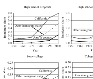
I begin the empirical analysis by describing how immigration affected different labor markets in the past few decades. As indicated earlier, most of the immigrants who entered the United States in the past 40 years have clustered in a relatively small number of states. Figure 1 shows the trends in the immigrant share, by educational attainment, for three groups of states: California, the other main immigrant-receiving states (Florida, Illinois, New Jersey, New York, and Texas), and the rest of the coun-try. Not surprisingly, the largest immigrant-induced supply increase occurred in California for the least-educated workers. By 2000, almost 80 percent of high school dropouts in California were foreign-born, as compared to only 50 percent in the other immigrant-receiving states, and 20 percent in the rest of the country. Although the scale of the immigrant influx is smaller for high-skill groups, there is still a large dis-parity in the size of the supply increase across the three areas. In 2000, for example, more than a quarter of college graduates in California were foreign-born, as compared to 18 percent in the other immigrant-receiving states, and 8 percent in the rest of the country.
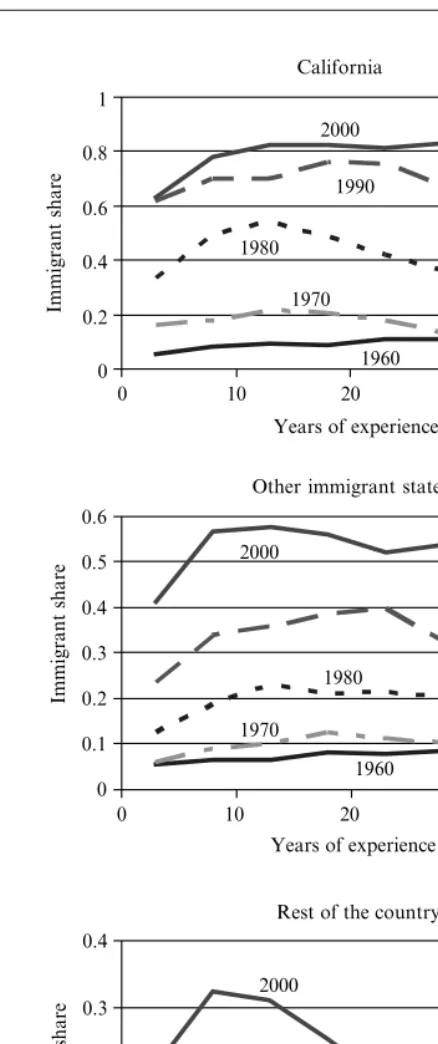
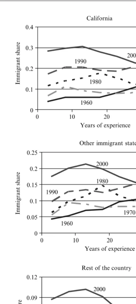
Figures 2 and 3 continue the descriptive analysis by showing the trends in the immigrant share for some of the specific schooling-experience groups used in the analysis. To conserve space, I only illustrate these profiles for the two education groups most affected by immigration: high school dropouts (Figure 2) and college graduates (Figure 3).
These figures show that there is significant dispersion in the relative size of the immigrant population over time and across experience groups, even when looking at a particular level of education and a particular part of the country. In 1980, for exam-ple, the immigration of high school dropouts in California was particularly likely to affect the labor market opportunities faced by workers with around 15 years of expe-rience, where around half of the relevant population was foreign-born. In contrast, only 30 percent of the workers with more than 30 years of experience were foreign-born. By 2000, however, more than 80 percent of all high school dropouts with between ten and 35 years of experience were foreign-born. These patterns differed in other parts of the country. In the relatively nonimmigrant rest of the country, immi-gration of high school dropouts was relatively rare prior to 1990, accounting for less than 10 percent of the workers in the relevant labor market. By 2000, however, immi-grants made up more than 30 percent of the high school dropouts with between five and 15 years of experience.
The data summarized in these figures, therefore, suggest that there has been a great deal of dispersion in how immigration affects the various skill groups in different regional labor markets. In some years, it affects workers in certain parts of the region-education-experience spectrum. In other years, it affects other workers. This paper Figure 1
The Immigrant Share of the Male Workforce, by Education and Area of Country Note: The “other immigrant states” include Florida, Illinois, New Jersey, New York, and Texas.
High school dropouts
1950 1960 1970 1980 1990 2000 Year
1950 1960 1970 1980 1990 2000 Year
1950 1960 1970 1980 1990 2000 Year
1950 1960 1970 1980 1990 2000 Year
Immigrant share
Rest of country Other immigrant states
California
0 0.4 0.6 0.8 1
0 10 20 30 40
Years of experience 1960 1970 1980
1990 2000
Immigrant share
Other immigrant states
0 0.1 0.2 0.3 0.4 0.6
0 10 20 30 40
Years of experience 1960 1970
1980
1990 2000
Immigrant share
Immigrant share
Rest of the country
0 0.1 0.2 0.3 0.4
0 10 20 30 40
Years of experience 1960
1970 1980
1990 2000 0.2
0.5
Figure 2
California
0 0.1 0.2 0.3 0.4
0 10 20 30 40
Years of experience
0 10 20 30 40
Years of experience
0 10 20 30 40
Years of experience
1960 1970
1980
1990 2000
Immigrant share
Immigrant share
Immigrant share
Other immigrant states
0 0.05 0.1 0.15 0.2 0.25
1960
1970 1980
1990
2000
Rest of the country
0 0.03 0.06 0.09 0.12
1960 1970
1980
1990
2000
Figure 3
exploits this variation to measure how wages and native worker migration decisions respond to immigration.
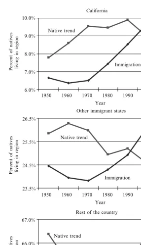
Before proceeding to a formal analysis, it is instructive to document that the raw data reveals equally strong differences in the way that natives have chosen to sort themselves geographically across the United States. More important, these location choices seem to be correlated with the immigrant-induced supply shifts. Figure 4 illustrates the aggregate trend. As first reported by Borjas, Freeman, and Katz (1997), the share of the native-born population that chose to live in California stopped grow-ing around 1970, at the same time that the immigrant influx began. This important trend is illustrated in the top panel of Figure 4. The data clearly show the relative num-bers of native workers living in California first stalling, and eventually declining, as the scale of the immigrant influx increased rapidly.21
The middle panel of Figure 4 illustrates a roughly similar trend in the other immi-grant states. As immigration increased in these states (the immiimmi-grant share rose from about 8 percent in 1970 to 22 percent in 2000), the fraction of natives who chose to live in those states declined slightly, from 26 to 24.5 percent.
Finally, the bottom panel of the figure illustrates the trend in the relatively nonim-migrant areas that form the rest of the country. Although immigration also increased over time in this region, the increase has been relatively small (the immigrant share rose from 2.5 percent in 1970 to 7.5 percent in 2000). At the same time, the share of natives living in this region experienced an upward drift, from 64.5 percent in 1970 to 66.5 percent in 2000. The evidence summarized in Figure 4, therefore, tends to sug-gest a link between native location decisions and immigration.
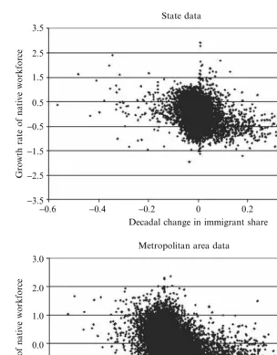
This link is also evident at more disaggregated levels of geography and skills. I used all of the Census data available between 1960 and 2000 to calculate for each (i, j) cell the growth rate of the native workforce during each decade (defined as the log of the ratio of the native workforce at the decade’s two endpoints) and the corre-sponding decadal change in the immigrant share. The top panel of Figure 5 presents the scatter diagram relating these decadal changes at the state level after removing decade effects. The plot clearly suggests a negative relation between the growth rate of a particular class of native workers in a particular state and immigration. The bot-tom panel of the figure illustrates an even stronger pattern when the decadal changes are calculated at the metropolitan area level. In sum, the raw data clearly reveal that the native workforce grew fastest in those labor markets that were least affected by immigration.
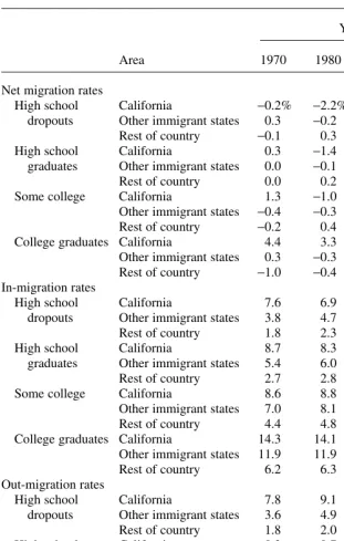
Finally, Table 1 provides an alternative way of looking at the data that also links native migration decisions and immigration. Beginning in 1970, the Census contains information not only on the person’s state of residence as of the Census date, but also on the state of residence five years prior to the survey. These data can be used to con-struct net-migration rates for each of the skill groups in each geographic market, as well as in-migration and out-migration rates. (The construction of these rates will be described in detail later in the paper.) To easily summarize the basic trends linking migration rates and immigration, I again break up the United States into three regions: California, the other immigrant-receiving states, and the rest of the country. A native
California
6.0% 7.0% 8.0% 9.0% 10.0%
1950 1960 1970 1980 1990 2000
Year
1950 1960 1970 1980 1990 2000
Year
1950 1960 1970 1980 1990 2000
Year Percent of natives living in region
Percent of natives living in region
Percent of natives living in region
6.0% 14.0% 22.0% 30.0% 38.0%
Immigrant share
Native trend
Immigration
Other immigrant states
23.5% 24.5% 25.5% 26.5%
6.0% 12.0% 18.0% 24.0%
Immigrant share
Native trend
Immigration
Rest of the country
64.0% 65.0% 66.0% 67.0%
0.0% 4.0% 8.0% 12.0% 16.0%
Immigrant share
Native trend
Immigration
Figure 4
Geographic Sorting of Native Workforce and Immigration
3.5
State data
2.5
Growth rate of native workforce
Growth rate of native workforce
1.5
0.5
−0.5
−1.5
−2.5
−3.5
−1.0
−2.0
−3.0
−0.6 −0.4
−0.5 −0.25 0 0.25 0.5 0.75
−0.2
3.0
2.0
1.0
0.0
Decadal change in immigrant share
Decadal change in immigrant share Metropolitan area data
0.2
0 0.4 0.6
Figure 5
Year
Area 1970 1980 1990 2000
Net migration rates
High school California −0.2% −2.2% −2.3% −5.4%
dropouts Other immigrant states 0.3 −0.2 −1.6 −1.4
Rest of country −0.1 0.3 0.8 1.0
High school California 0.3 −1.4 −0.8 −4.5
graduates Other immigrant states 0.0 −0.1 −0.8 −0.9
Rest of country 0.0 0.2 0.4 0.7
Some college California 1.3 −1.0 0.3 −3.4
Other immigrant states −0.4 −0.3 −0.9 −0.8
Rest of country −0.2 0.4 0.3 0.9
College graduates California 4.4 3.3 4.5 1.9
Other immigrant states 0.3 −0.3 −0.8 −0.4 Rest of country −1.0 −0.4 −0.5 −0.1 In-migration rates
High school California 7.6 6.9 6.2 4.0
dropouts Other immigrant states 3.8 4.7 4.5 4.2
Rest of country 1.8 2.3 2.6 2.5
High school California 8.7 8.3 7.7 4.9
graduates Other immigrant states 5.4 6.0 5.2 4.6
Rest of country 2.7 2.8 2.6 2.5
Some college California 8.6 8.8 7.8 5.3
Other immigrant states 7.0 8.1 6.7 6.2
Rest of country 4.4 4.8 4.0 3.6
College graduates California 14.3 14.1 13.0 11.1
Other immigrant states 11.9 11.9 10.0 9.4
Rest of country 6.2 6.3 5.4 4.8
Out-migration rates
High school California 7.8 9.1 8.5 9.5
dropouts Other immigrant states 3.6 4.9 6.1 5.6
Rest of country 1.8 2.0 1.9 1.6
High school California 8.3 9.7 8.5 9.5
graduates Other immigrant states 5.4 6.1 6.0 5.5
Rest of country 2.7 2.6 2.3 1.7
Some college California 7.3 9.8 7.5 8.7
Other immigrant states 7.4 8.4 7.6 7.0
Rest of country 4.6 4.4 3.7 2.8
College graduates California 9.9 10.8 8.4 9.2
Other immigrant states 11.7 12.1 10.8 9.8
Rest of country 7.2 6.7 5.9 4.9
worker is then defined to be an internal migrant if he moves across these three regions in the five-year period prior to the Census.
The differential trends in the net-migration rate across the three regions are reveal-ing. Within each education group, there is usually a steep decline in the net migration rate into California, a slower decline in the net migration rate into the other immigrant states, and a slight increase in the net migration rate into the rest of the country. In other words, the net migration of natives fell most in those parts of the country most heavily hit by immigration.
The other panels of Table 1 show that the relative decline in net migration rates in the immigrant-targeted states arises because of both a relative decline in the in-migration rate and a relative increase in the out-migration rate. For example, the in-migration rate of native high school dropouts into California fell from 7.6 to 4.0 percent between 1970 and 2000, as compared to a respective increase from 1.8 to 2.5 percent in the rest of the country. Similarly, the out-migration rates of high school dropouts rose from 7.8 to 9.5 percent in California and from 3.6 to 5.6 per-cent in the other immigrant states, but fell from 1.8 to 1.6 perper-cent in those states least hit by immigration.
IV. Immigration and Wages
In earlier work (Borjas 2003), I showed that the labor market impact of immigration at the national level can be estimated by examining the wage evo-lution of skill groups defined in terms of educational attainment and experience. This section of the paper reestimates some of the models presented in my earlier paper, and documents the sensitivity of the wage impact of immigration to the geographic definition of the labor market.
I measure the wage impact of immigration using four alternative definitions for the geographic area covered by the labor market. In particular, I assume that the labor market facing a particular skill group is: (1) a national labor market, so that the wage impact of immigration estimated at this level of geography presumably measures the factor price elasticity ηin the model; (2) a labor market defined by the geographic boundaries of the nine Census divisions; (3) a labor market that operates at the state level; or (4) a labor market bounded by the metropolitan area.22
Let log wijtdenote the mean log weekly wage of nativemen who have skills i, work
in region j, and are observed at time t.23I stack these data across skill groups, geo-graphic areas, and Census cross-sections and estimate the model:
(14) log wijt= θWpijt+si+rj+ πt+(si×rj) +(si× πt) +(rj× πt) + ϕijt,
where siis a vector of fixed effects indicating the group’s skill level; rjis a vector of
fixed effects indicating the geographic area of residence; and πtis a vector of fixed
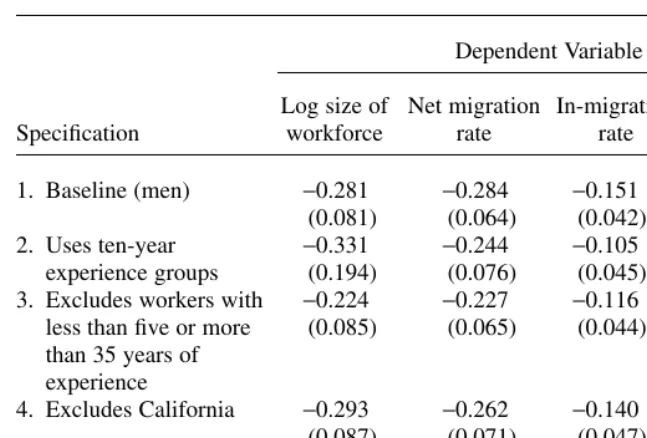
22. The metropolitan area is defined in a roughly consistent manner across Censuses beginning in 1980. The analysis conducted at the metropolitan area level, therefore, uses only the 1980–2000 cross-sections and excludes all workers residing outside the identifiable metropolitan areas.
effects indicating the time period of the observation. The linear fixed effects in Equation 14 control for differences in labor market outcomes across skill groups and regions, and over time. The interactions (si × πt) and (sj × πt) control for secular
changes in the returns to skills and in the regional wage structure during the 1960-2000 period. Finally, the inclusion of the interactions (si×rj) implies that the
coeffi-cient θWis being identified from changes in wages and immigration that occur within
skill-region cells.
Note that the various vectors of fixed effects included in Equation 14 correspond to the vectors of fixed effects implied by the estimating equation derived from the model (Equation 12). The only exception is that Equation 14 also includes interactions between region and Census year. These interactions would clearly enter the theory if demand shocks were allowed to differentially affect regions over time.
The regression coefficients reported in this section come from weighted regres-sions, where the weight is the sample size used to calculate the mean log weekly wage in the (i, j, t) cell.24The standard errors are clustered by skill-region cells to adjust for the possible serial correlation that may exist within cells.
Finally, the specification I use in the empirical analysis uses the immigrant share, p, rather than the relative number of immigrants as of time t, m~= M~/N, as the measure
of the immigrant-induced supply increase. It turns out that the relation between the various dependent variables and the relative number of immigrants is highly nonlin-ear, and is not captured correctly by a linear term in m~. The immigrant share approx-imates log m~, so that using the immigrant share introduces some nonlinearity into
the regression model. In fact, the wage effects (appropriately calculated) are similar when including either log m~or a second-order polynomial in m~as the measure of the
immigrant supply shift.25
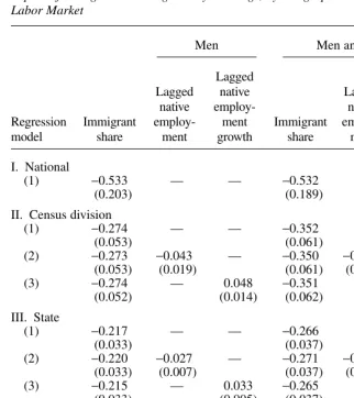
Consider initially the first three columns of Table 2, which present the basic estimates of the adjustment coefficient θWobtained from the sample of working men.
The first row summarizes the regression results when the geographic reach of the labor market is assumed to encompass the entire nation.26The estimated coefficient is −0.533, with a standard error of 0.203. It is easier to interpret this coefficient by converting it to an elasticity that gives the percent change in wages associated with a percent change in labor supply. In particular, define the wage elasticity as:
(15) ~ ~
24. The coefficients of the immigrant share variable are quite similar when the regressions are not weighted. 25. To illustrate, a regression of the log weekly wage on the relative number of immigrants variable m~
(and all the fixed effects) has a coefficient of −0.160 (with a standard error of 0.082). The same regression on the log of the relative number variable has a coefficient of −0.071 (.027). Evaluated at the mean value of m~
By 2000, immigration had increased the size of the workforce by 17.2 percent. Equation 15 implies that the wage elasticity—evaluated at the mean value of the rel-ative number of immigrants—can be obtained by multiplying θWby 0.73. The wage
elasticity for weekly earnings is then −0.39 (or −0.532 ×0.73). Put differently, a 10 percent immigrant-induced supply increase—that is, an immigrant flow that increases the number of workers in a skill group by 10 percent—reduces weekly earnings in that group by almost 4 percent.
Suppose now that the worker’s state of residence defines the geographic area encom-passed by the labor market. The data then consists of stacked observations on the immigrant share and the mean log weekly wage for cell (i, j, t). The first row of Panel III in Table 2 reports the estimated coefficient of the immigrant share variable when Equation 14 is estimated at the state level. The adjustment coefficient is –0.217, with a standard error of 0.033. At the mean immigrant-induced supply shift, the state-level regression implies that a 10 percent increase in supply reduces the native wage by only 1.6 percent, roughly 40 percent of the estimated impact at the national level. Note that the derivative in Equation 15 is precisely the wage impact of immigration captured by the region-specific immigrant stock variable in Equation 12. In terms of the parameters of the theoretical model, this derivative estimates the product of elasticities .η(1 + ση). As discussed earlier, the model suggests that the log wage regression—when esti-mated at the local labor market level—should include a variable that approximately measures the lagged relative number of natives who would have migrated in the absence of immigration. The second row of the panel adds a variable giving the log of the size of the native workforce ten years prior to the Census date.27The inclusion of lagged employment does not alter the quantitative nature of the evidence. The adjustment coefficient is −0.220 (0.033). Finally, the third row of the panel introduces an alternative variable to control for the counterfactual native migration flow, namely the rate of growth in the size of the native workforce in the ten-year period prior to the census date. Again, the estimated wage effects are quite similar.
The remaining panels in Table 2 document the behavior of the coefficient θWas
the geographic boundary of the labor market is either expanded (to the Census divi-sion level) or narrowed (to the metropolitan area level). The key result implied by the comparison of the various panels is that the adjustment coefficient grows numeri-cally larger as the geographic reach of the labor market expands. Using the simplest specification in Row 1 in each of the panels, for example, the adjustment coefficient is −0.043 (0.025) at the metropolitan area level, increases to −0.217 (0.033) at the state level, increases further to −0.274 (0.053) at the division level, and jumps to −0.533 (0.203) at the national level.
Up to this point, I have excluded working women from the analysis because of the inherent difficulty in measuring their labor market experience and classifying them correctly into the various skill groups. Nevertheless, the last three columns of Table 2 replicate the entire analysis using both working men and women in the regression models. The national-level coefficient is almost identical to that obtained when the regression analysis used only working men. Equally important, the regressions reveal
Table 2
Impact of Immigration on Log Weekly Earnings, by Geographic Definition of the Labor Market
Men Men and women
Lagged Lagged
Lagged native Lagged native
native employ- native
employ-Regression Immigrant employ- ment Immigrant employ- ment
model share ment growth share ment growth
I. National
(1) −0.533 — — −0.532 — —
(0.203) (0.189)
II. Census division
(1) −0.274 — — −0.352 — —
(0.053) (0.061)
(2) −0.273 −0.043 — −0.350 −0.040 —
(0.053) (0.019) (0.061) (0.017)
(3) −0.274 — 0.048 −0.351 — 0.048
(0.052) (0.014) (0.062) (0.015)
III. State
(1) −0.217 — — −0.266 — —
(0.033) (0.037)
(2) −0.220 −0.027 — −0.271 −0.033
(0.033) (0.007) (0.037) (0.007)
(3) −0.215 — 0.033 −0.265 — 0.035
(0.033) (0.005) (0.037) (0.006)
IV. Metropolitan area
(1) −0.043 — — −0.057 — —
(0.025) (0.024)
(2) 0.021 −0.016 — −0.001 −0.010 —
(0.048) (0.012) (0.051) (0.012)
(3) 0.048 — 0.030 0.024 — 0.030
(0.047) (0.008) (0.050) (0.008)
the same clear pattern of a numerically smaller adjustment coefficient as the labor market becomes geographically smaller: from −0.352 (0.061) in the division-level regression to −0.266 (0.037) in the state-level regression to −0.057 (0.024) in the regressions estimates at the level of the metropolitan area. The results, therefore, are quite robust to the inclusion of working women.
The theoretical model presented earlier suggests an interesting interpretation for this correlation between the geographic size of the labor market and the measured wage effect of immigration. As the geographic region becomes smaller, there is more spatial arbitrage—due to interregional flows of labor—that tends to equalize opportu-nities for workers of given skills across regions.
An alternative explanation for the pattern is that the smaller wage effects measured in smaller geographic units may be due to attenuation bias. The variable measuring the immigrant stock will likely contain more measurement errors when it is calculated at more disaggregated levels of geography. As I show in the next section, it is unlikely that attenuation bias can completely explain the monotonic relation between the adjustment coefficient and the geographic reach of the labor market.
Overall, the evidence seems to indicate that even though immigration has a sizable adverse effect on the wage of competing workers at the national level, the analysis of wage differentials across regional labor markets conceals much of that impact. The remainder of this paper examines whether these disparate findings can be attributed to native internal migration decisions.
V. Immigration and Internal Migration
I now estimate a variety of models—closely linked to the theoretical discussion in Section II—to determine if the evolution of the native workforce or the internal migration behavior of natives is related to immigrant-induced supply increases in the respective labor markets.
A. The Size of the Native Workforce
Consider the following regression model:
(16) log Nijt= Xijt β + θNPijt+si+rj+ πt+(si× πt) +(rj× πt) +(si×rj) + εijt,
where Xis a vector of control variables discussed below. As with the wage regression specified earlier, the various vectors of fixed effects absorb any region-specific, skill-specific, and time-specific factors that affect the evolution of the native workforce in a particular labor market. Similarly, the interactions allow for decade-specific changes in the number of workers in particular skill groups or in particular states caused by shifts in aggregate demand. Finally, the interaction between the skill and region fixed effects implies that the coefficient of the immigrant supply variable is being identified from changes that occur within a specific skill-region grouping. As before, all stan-dard errors are adjusted for any clustering that may occur at the skill-region level.28
I again estimate the model using three alternative definitions for the geographic area encompassed by the labor market: a Census division, a state, and a metropolitan area. Table 3 presents alternative sets of regression specifications that show how the immi-grant-induced supply shift affects the evolution of the size of the native workforce.
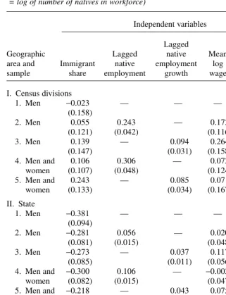
Consider initially the regressions estimated at the state level, reported in the mid-dle panel of the table. The specification in Row 1 uses the sample of working men and does not include any variables in the vector X. The estimated coefficient of the immi-grant share variable is −0.381, with a standard error of 0.094. This regression model, therefore, confirms that there is a numerically important and statistically significant negative relation between immigration and the rate of growth of the native workforce at the state level. The coefficient is easier to interpret by calculating the derivative
/ , N M
2 2 ~ which gives the change in the size of the native workforce when the stock of
immigrant workers increases by one. It is easy to show that the derivative of interest is:
(17) ~ ~
As before, the derivative in Equation 17 can be evaluated at the mean value of the immigrant supply increase by multiplying the regression coefficient θNby 0.73. The
simplest specification reported in Panel II of Table 3 implies that 2.8 fewer native workers chose to live in a particular state for every ten additional immigrants entering that state. In terms of the theoretical model, Equation 11 implies that the derivative reported in Equation 17 estimates the product of elasticities ησ.
The next two rows of the middle panel of Table 3 estimate more general specifica-tions of the regression model. As noted earlier, I adjust for preexisting migration flows by including either the lagged log of the number of native workers or the lagged rate of growth in the size of the native workforce.29I also include variables measuring the mean log weekly wage and the unemployment rate in the labor market (again meas-ured at the state level).30These additional variables control for factors that, in addi-tion to immigraaddi-tion, motivate income-maximizing native workers to move from one market to another.
Rows 2 and 3 yield very similar results, so the evidence is not sensitive to which variable is chosen to proxy for the lagged size of native net migration in the absence of immigration. Not surprisingly, lagged measures of the size of the native workforce
(due to the presence of sampling weights in the 1990 and 2000 Censuses). A weighted regression is prob-lematic because it introduces a strong positive correlation between the weight and the dependent variable (observations with large values of the dependent variable would mechanically count more in the regression analysis), and errors in the measurement of the dependent variable would be amplified by the weighting scheme. This type of nonclassical measurement error, which has not been appreciated sufficiently in previ-ous studies, imparts a positive bias on the adjustment coefficient in Equation 16. In fact, a weighted regression of the state-level specification reported in Row 1 of Table 3 leads to an adjustment coefficient of −0.135 (0.094).
29. To avoid reintroducing the dependent variable on the right-hand-side, the regressions presented in this section use the lagged growth rate of the native workforce ten to 20 years prior to the Census date. For exam-ple, the lagged growth rate for the observation referring to high school graduates in Iowa in 1980 would be the growth rate in the number of high school graduates in Iowa between 1960 and 1970. This definition of the lagged growth rate implies that the regression models using this specification do not include any cells drawn from the 1960 Census.
Table 3
Impact of Immigration on the Size of the Native Workforce (Dependent variable = log of number of natives in workforce)
Independent variables
Lagged
Geographic Lagged native Mean
area and Immigrant native employment log Unemployment
sample share employment growth wage rate
I. Census divisions
1. Men −0.023 — — — —
(0.158)
2. Men 0.055 0.243 — 0.172 −1.327
(0.121) (0.042) (0.116) (0.437)
3. Men 0.139 — 0.094 0.264 −1.485
(0.147) (0.031) (0.158) (0.529)
4. Men and 0.106 0.306 — 0.072 −1.282
women (0.107) (0.048) (0.124) (0.402)
5. Men and 0.243 — 0.085 0.071 −1.816
women (0.133) (0.034) (0.167) (0.483)
II. State
1. Men −0.381 — — — —
(0.094)
2. Men −0.281 0.056 — 0.020 −0.376
(0.081) (0.015) (0.048) (0.194)
3. Men −0.273 — 0.037 0.117 −0.635
(0.085) (0.011) (0.056) (0.208)
4. Men and −0.300 0.106 — −0.002 −0.597
women (0.082) (0.015) (0.047) (0.176)
5. Men and −0.218 — 0.043 0.075 −0.611
women (0.083) (0.011) (0.054) (0.184)
III. Metropolitan area
1. Men −0.785 — — — —
(0.060)
2. Men −0.839 −0.402 — 0.072 −0.307
(0.091) (0.022) (0.044) (0.151)
3. Men and −0.712 −0.365 — 0.057 −0.237
women (0.087) (0.021) (0.044) (0.125)
or its growth rate have a positive impact on the current number of native workers. Similarly, the mean log wage has a positive (sometimes insignificant) coefficient, while the unemployment rate has a negative effect. The coefficient of the immigrant share variable falls to around −0.27 in the most general specification.31This estimate implies that around two fewer native workers choose to reside in a particular state for every ten additional immigrants who enter that state.
The final two rows of the middle panel add the population of working women to the regression analysis. These regressions, in effect, examine the evolution of the entire workforce for a particular labor market defined by skills and region. The inclu-sion of women in this type of regresinclu-sion model could be problematic because of the possibility that many women may be tied movers or tied stayers, so that their location decisions may crucially depend on factors (such as family composition and the distri-bution of skills within the family) that are ignored in the study. Nevertheless, the state-level regressions suggest that, at least qualitatively, the inclusion of women barely alters the results. The coefficients of the immigrant share variable are not only nega-tive and statistically significant, but are also roughly similar to the ones estimated in the sample of working men.
The other panels of Table 3 reestimate the regression models at the census division and metropolitan area levels. The estimated impact of the immigrant supply variable typically has the wrong sign at the division level, but with large standard errors. In contrast, the adjustment coefficient is very negative (and statistically significant) at the metropolitan area level. The obvious conclusion to draw by comparing the three pan-els of the table is that the negative impact of the immigrant share variable gets numer-ically stronger the smaller the geographic boundaries of the labor market. In the general specification reported in Row 2 for working men, for example, the estimated coefficient of the immigrant share variable is 0.055 (0.121) at the Census division level; −0.281 (0.081) at the state level; and −0.839 (0.091) at the metropolitan area level.32The coefficient of the metropolitan area regression, in fact, implies that 6.1 fewer native workers choose to reside in a particular metropolitan area for every ten additional immigrants who enter that locality.
It is worth noting that the geographic variation in the observed spatial correlation between the size of the native workforce and immigration is an exact mirror image of the geographic variation in the spatial correlation between wages and immigration reported in Table 2. As implied by the model, the wage effects are larger when the impact of immigration on the size of the native workforce is weakest (at the Census division level); and the wage effects are weakest when the impact of immigration on the size of the native workforce is largest (at the metropolitan area level).
It would seem as if this mirror-image pattern is not consistent with an attenuation hypothesis: more measurement error for data estimated at smaller geographic units would lead to smaller coefficient estimates at the metropolitan area level in both Tables 2 and 3. There is, however, one possible source of measurement error that could potentially explain the mirror-image pattern. In particular, note that the
31. The coefficient would be virtually identical if both the lagged level and growth rate of the native work-force were included in the regression.
adjustment coefficient θNestimated by Equation 16 may suffer from division bias.
The dependent variable appears (in transformed form) as part of the denominator in the immigrant share variable. If the size of the native workforce were measured with error, the division bias would lead to downward-biased estimates of the adjustment coefficient. One could argue that such measurement error would be more severe at the metropolitan area level than in larger geographic regions.
I show below, however, that division bias does not play a central role in generating the mirror-image pattern of coefficients in Tables 2 and 3. Instead, the mirror-image pattern revealed by the two tables provides some support for the hypothesis that there is indeed a behavioral response by the native population that is contaminating the measured wage impact of immigration on local labor markets.
B. Migration Rates
Since 1970 the census contains detailed information on the person’s state of resi-dence five years prior to the census, and since 1980 there is similar information for the metropolitan area of residence. These data, combined with the information on geographic location at the time of the census, can be used to compute in-, out-, and net-migration rates for native workers in the various skill-region groups. I now exam-ine how these native migration rates respond to the immigrant influx. Therefore, the results presented in this section, which examine the flows of actualnative movers, can be interpreted as providing independent confirmation of the findings presented above that link the evolution of the size of the native workforce to the immigrant influx.
To illustrate the calculation of the net migration rate, consider the data available at the state level in a particular census. The worker is an out-migrant from the “original” state of residence (that is, the state of residence five years prior to the survey) if he lives in a different state by the time of the census. The worker is an in-migrant into the current state of residence if he lived in a different state five years prior to the cen-sus. I define the in-migration and out-migration rates by dividing the total number of in-migrants or out-migrants in a particular skill-state-time cell by the relevant work-force in the baseline state.33The net migration rate is then defined as the difference between the in-migration and the out-migration rate. To make the results in this sec-tion comparable to those reported in Table 3, I multiply all the migrasec-tion rates by two—this adjustment converts the various rates into decadal changes (which was the unit of change implicitly used in the native workforce regressions).
I concluded the presentation of the theoretical model in Section II by deriving estimable equations that related the size of the native workforce and the native wage to the immigrant supply shift. This section uses a variation of the model with a dif-ferent dependent variable. Equation 7 gives the expression for the net migration rate
for cell (i, j, t). By using the approximation that (1 +x)t≈1 +xt, the equation
deter-mining the net-migration rate, vijt, can be rewritten as:
(18) vijt= ησ λij+(ησ)2(tλij) − ησm ~
it+ ησm
~ ijt.
As before, the regression model that I actually use to analyze how migration rates respond to immigration is:
(19) yijt= Xijtβ + θNPijt+si+rj+ πt+(si× πt) +(rj× πt) +(si×rj) + εijt,
where yijtrepresents the net-migration, in-migration, or out-migration rate for cell
(i, j, t). Note that the coefficient of the region-specific immigrant share variable θN
identifies the product of elasticities ησ.
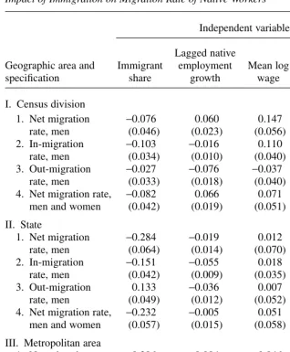
Table 4 summarizes the evidence. To conserve space, I only report the general spec-ification that includes all of the variables in the vector X. Consider initially the regres-sion results reported for the sample of working men in Panel II, where the dependent variable is the net migration rate estimated at the state level. Because the depend-ent variable in this regression model measures a changein the native population, I use the lagged native employment growth rate as a preferred way of controlling for preexisting conditions.34 The estimated coefficient of the immigrant share variable in the net migration regression is −0.284, with a standard error of 0.064. As before, this coefficient is more easily interpretable by multiplying it by 0.73, indicating that 2.1 fewer native workers (on net) move to a particular state for every ten immigrants who enter that state. It is worth noting that the estimated product of elasticities ησis very similar to the corresponding estimate reported in Table 3, when the dependent variable was the log of the size of the native workforce.
Rows 2 and 3 of the middle panel show that the effect of immigration on net migra-tion rates arises both because immigramigra-tion induces fewer natives to move into the immigrant-penetrated labor markets, and because immigration induces more natives to move out of those markets. The coefficient of the immigrant share variable in the in-migration regression is −0.151 (0.042), while the respective coefficient in the out-migration regression is 0.133 (0.049). In rough terms, an influx of ten immigrants into a state’s workforce induces one fewer native worker to migrate there and encourages one native worker already living there to move out.
Finally, the last row in the middle panel replicates the net migration rate regres-sion in the sample of workers that includes both men and women. The adjustment coefficient is negative and significant (−0.232, with a standard error of 0.057). As before, the inclusion of women into the analysis does not fundamentally change the results.
The top and bottom panels of Table 4 reproduce the earlier finding that the nega-tive impact of immigration on nanega-tive migration rates is numerically larger as the geo-graphic area that encompasses the labor market becomes smaller. In the sample of working men, the estimated coefficient of the immigrant share variable on the net migration rate is −0.076 (0.046) at the division level; −0.284 (0.064) at the state level;
Table 4
Impact of Immigration on Migration Rate of Native Workers
Independent variable Lagged native
Geographic area and Immigrant employment Mean log Unemployment
specification share growth wage rate
I. Census division
1. Net migration −0.076 0.060 0.147 −0.048
rate, men (0.046) (0.023) (0.056) (0.206)
2. In-migration −0.103 −0.016 0.110 0.151
rate, men (0.034) (0.010) (0.040) (0.143)
3. Out-migration −0.027 −0.076 −0.037 0.200
rate, men (0.033) (0.018) (0.040) (0.165)
4. Net migration rate, −0.082 0.066 0.071 0.059
men and women (0.042) (0.019) (0.051) (0.189)
II. State
1. Net migration −0.284 −0.019 0.012 0.242
rate, men (0.064) (0.014) (0.070) (0.216)
2. In-migration −0.151 −0.055 0.018 0.026
rate, men (0.042) (0.009) (0.035) (0.127)
3. Out-migration 0.133 −0.036 0.007 −0.216
rate, men (0.049) (0.012) (0.052) (0.171)
4. Net migration rate, −0.232 −0.005 0.051 −0.125
men and women (0.057) (0.015) (0.058) (0.187)
III. Metropolitan area
1. Net migration −0.396 −0.084 −0.046 0.094
rate, men (0.086) (0.015) (0.042) (0.137)
2. In-migration −0.114 −0.077 −0.018 0.054
rate, men (0.057) (0.009) (0.027) (0.092)
3. Out-migration 0.282 0.007 0.028 −0.041
rate, men (0.062) (0.010) (0.028) (0.095)
4. Net migration rate, −0.336 −0.093 −0.057 0.029
men and women (0.073) (0.015) (0.037) (0.104)