Michael F. Lovenheim is an assistant professor of policy analysis and management at Cornell University as well as a faculty research fellow at the National Bureau of Economic Research. C. Lockwood Reynolds is an assistant professor of economics at Kent State University. The authors wish to thank John Bound, Charlie Clotfelter and Caroline Hoxby for helpful comments on this paper as well as seminar participants at Cornell University, MIT, the University of Texas–Dallas, the University of Akron, the National Bureau of Economic Research Household Finance Meeting, and the American Education Finance Association Annual Meeting. Jen Doleac provided excellent research assistance. The authors also thank the Stanford Institute for Economic Policy Research (SIEPR) and the Pew Charitable Trust Economic Mobility Project for
fi nancial support for this project. The data used in this article can be obtained beginning July 2013 through June 2016 from the author.
[Submitted April 2011; accepted April 2012]
022 166X E ISSN 1548 8004 8 2013 2 by the Board of Regents of the University of Wisconsin System
T H E J O U R N A L O F H U M A N R E S O U R C E S • 48 • 1
The Effect of Housing Wealth on
College Choice
Evidence from the Housing Boom
Michael F. Lovenheim
C. Lockwood Reynolds
A B S T R A C T
We use NLSY97 data to examine how home price variation affects the quality of postsecondary schools students attend. We fi nd a $10,000 increase in housing wealth increases the likelihood of public fl agship university enrollment relative to nonfl agship enrollment by 2.0 percent and decreases the relative probability of attending a community college by 1.6 percent. These effects are driven by lower- income families, predominantly by altering student application decisions. We also fi nd home price changes affect direct quality measures of institutions students attend. Furthermore, for lower- income students, each $10,000 increase in home prices leads to a 1.8 percent increase in the likelihood of completing college.
I. Introduction
The Journal of Human Resources 2
2012).1 The higher level of resources at elite public and private institutions also trans-late into more favorable student outcomes, including higher completion rates (Bound, Lovenheim, and Turner 2010) and lower time to degree (Bound, Lovenheim, and Turner 2012). Furthermore, there is considerable evidence that the type of institution in which students initially enter the postsecondary education system affects the likeli-hood of graduation and future wages.2
Given these large returns to college quality, little work has been done examining how students make decisions about which college to attend and, in particular, what role household fi nances play in this decision. There is ample evidence that low- income students are under- represented at elite private and state fl agship universities (Bowen, Kurzweil, and Tobin 2005; Pallais and Turner 2006, 2007). Using the National Longi-tudinal Survey of Youth (NLSY), previous work has estimated sizable income gradi-ents in the two- year, four- year decision as well as in four- year college quality (Belley and Lochner 2007; Kinsler and Pavan 2010)3 and has shown that higher- income stu-dents attend schools with higher SAT scores (Light and Strayer 2000). There also is evidence that students are highly responsive to college- quality differences among institutions (Long 2004; Avery and Hoxby 2004). Though informative of many of the factors that infl uence college choices, there still is a poor understanding of the causal effect of household resources on the college- quality decisions of students.
This paper examines how household resources infl uence the quality of postsec-ondary schools in which students enroll, focusing specifi cally on the role of housing wealth because of the central importance of this form of wealth to the majority of families. For most American families, the home is the largest single asset, and for many households it is their only substantial asset. For example, in the 2004 Survey of Consumer Finances, 48 percent of homeowners had less than $10,000 in nonhousing assets. Among homeowners with adjusted gross income (AGI) less than $75,000, the median nonhousing wealth amount was $6,300. Median home equity among these households was $80,000. In contrast, for households with AGI more than $125,000, median nonhousing wealth was $146,600 and median home equity was $293,500. Thus, for the lower and middle class, housing wealth is an extremely important com-ponent of total resources. An additional reason to focus on housing wealth is that there has been substantial variation in home prices in recent years that we argue generates exogenous variation in household fi nances.
1. Dale and Krueger (2002) fi nd no return to attending a higher average SAT university overall but show sizeable impacts for students from lower- income families. All of the studies estimating the returns to educa-tion quality are subject to identifi cation concerns (Hoxby 2009) but the identifi cation assumptions across studies vary suffi ciently that the sum total of the evidence points strongly to a signifi cant earnings return to college quality.
2. For evidence on the negative effect of beginning college at a two- year school, see Reynolds (2012), Kurlaender and Long (2009), and Rouse (1995). Bound, Lovenheim, and Turner (2010) also show that even conditional on institutional resources, BA completion rates are much lower at community colleges and less selective four- year public schools than at elite public and private institutions. Light and Strayer (2000) show similar negative effects on the likelihood of graduating from attending schools lower in the SAT score distri-bution—although they additionally highlight the importance of “match quality” between the quality of the school and the academic preparation of the student.
Lovenheim and Reynolds 3
We use a virtually identical source of variation in home prices as Lovenheim (2011) and Lovenheim and Mumford (forthcoming), which exploits differences across cities over time in the size and timing of the housing boom to identify how housing wealth infl uences postsecondary choices. Lovenheim (2011) shows that students who came of college age in areas that experienced recent large home price increases are more likely to go to college, while Lovenheim and Mumford show that female homeowners who experience home price growth are more likely to have a child. Although both of these papers exploit the same source of home price variation as used in this analysis, we make several contributions to the existing literature. First, we focus on identifying the impact of housing wealth on the quality of schools students attend (the intensive margin) rather than on the extensive margin. We estimate the effect of housing wealth on the likelihood a student attends a fl agship public university, a private university, or a two- year college, all relative to the likelihood of enrolling in a nonfl agship public university. This is the fi rst paper to explicitly estimate how family resources affect students’ choices between all of the different types of schools available to them, rather than focusing only on the two- year, four- year margin or on the extensive margin of college enrollment. Second, both Lovenheim (2011) and Lovenheim and Mumford (forthcoming) use the Panel Study of Income Dynamics (PSID). While the PSID has detailed housing wealth data, it does not contain rich information on college en-rollment timing or on precollegiate academic ability. The current analysis uses the NLSY97, which allows us to examine how sensitive the results in Lovenheim (2011) are to the inclusion of student ability measures as well as to the use of another sample. Third, our use of the NLSY97 allows us to dig more deeply into the ways in which housing wealth infl uences postsecondary choices and student outcomes. We estimate the effect of home price variation on student application decisions, the delay between high school and college, BA receipt, and student labor supply while enrolled in col-lege. These outcomes provide a more complete picture of how wealth in general and housing wealth in particular affect students’ paths through the postsecondary system.
Finally, the majority of previous work examining college choices and family re-sources, such as Kinsler and Pavan (2010), estimates conditional income gradients. Instead, we use quasi- experimental variation in home prices generated by the most recent housing boom to identify the effect of household wealth on college choice. Our approach allows one to assess the validity of the assumption made in the income gradient literature that income is conditionally exogenous. Furthermore, how housing wealth variation infl uences the intensive margin of college choice is of high policy interest in its own right given the evidence suggesting large labor market and educa-tional returns to attending different types of colleges combined with the large fl uctua-tions in home prices in the United States over the past decade. The decision of where to go to college may be at least as important for future labor market outcomes as is the decision of whether to attend college,4 so identifying how family resources in general and housing wealth in particular affect college choices on the intensive margin is of central importance.
We quantify the effect of individual- level home price growth that is driven by MSA-
The Journal of Human Resources 4
level home price changes on college choice using restricted- use NLSY97 data that provide detailed information on postsecondary institutions attended and the Metro-politan Statistical Area (MSA) in which the student’s family lived in 1997 as well as AFQT scores and student demographic characteristics. We estimate multinomial logit models among homeowners of the likelihood of attending a fl agship state university, a private university, or a community college, with nonfl agship public four- year schools as the omitted category, as a function of home price growth in the four years prior to a student turning 18. We also control for a detailed set of student background charac-teristics that include AFQT scores and state fi xed effects. Our empirical strategy is to compare the college choices of students within states or cities who come of college age in different years and thus who experience housing price increases of varying magnitudes when they are in high school. The main identifying assumptions are that housing price changes at the state or MSA level as well as initial home price and homeownership status are conditionally exogenous. We present detailed evidence that our results are robust to these assumptions.
We fi nd that home price variation affects college quality. A $10,000 increase in home prices in the four years prior to turning 18 increases the relative probability of attending a public fl agship by 0.0019 percentage points, or 2.0 percent, and decreases the probability of attending a community college by 0.0059 percentage points, or 1.6 percent. We split our sample into three income groups and fi nd that the effect of short- run housing wealth changes on enrollment decisions is largest for students from lower and middle- class households earning less than $75,000 per year. Similar to Lovenheim (2011), we also fi nd that home price changes affect the extensive margin of college enrollment, and we show these results are robust to including controls for precollegiate academic ability.
The changes in college- sector choices we fi nd suggest that students are reacting to home price changes by altering application and enrollment decisions. Using applica-tion data, we show that home price changes lead to increases in the total number of applications and to applications to both fl agship and nonfl agship four- year schools. However, conditional on applying, there is no strong relationship between home price changes and admission, which suggests that the college- sector effects we estimate are coming from changes in student behavior, not from changes in institutional admissions decisions.
The effect of home price changes on selection across sectors leads to increases in observable institutional quality and resources for affected students. These effects also are largest for families with household income below $75,000 per year. Finally, we present evidence that short- run housing price growth in the time period prior to children being of college age is positively associated with the likelihood of obtaining a BA for the lowest- income households in our sample, increasing BA attainment rates by 1.8 percent for each $10,000 increase in home prices during high school. Labor supply is negatively affected by home price growth as well, which together with the school quality effect likely drives the BA result.
Lovenheim and Reynolds 5
and previous literature present evidence they do, the burst of the housing bubble could have long- run consequences for the national stock of college- educated labor.
II. Data
A. NLSY97 Data
The data we use for this analysis come from the restricted- access National Longitudi-nal Survey of Youth 1997 (NLSY97), which is a natioLongitudi-nally- representative survey of children age 12 through 18 in 1997. Respondents are interviewed initially in 1997 and then yearly thereafter until 2008, which is the most recent follow- up available.
The NLSY97 data contain detailed family background and student demographic information, including parental education levels, family income in 1997, and home value. For mother’s and father’s education, we include dummy variables indicating highest level of schooling completed: no high school diploma, high school diploma (or GED), some college, and BA or more. One of the major advantages of the NLSY97 is that respondents were given the Armed Forces Qualifying Test (AFQT) in 1997, which is a comprehensive test of cognitive skills. Together with controls for parental educa-tion and income, these test scores allow us to control for the ability level of students, which is correlated with college choices and potentially with housing price growth.
The NLSY97 data include a signifi cant amount of item nonresponse. For example, 10.8 percent of the sample does not have a valid father’s education level, approxi-mately 16.6 percent of the sample is missing family income information and 23 per-cent of respondents do not have valid AFQT scores. Many previous analyses drop respondents without valid income and AFQT scores (Belley and Lochner 2007; Cam-eron and Taber 2004; Carneiro and Heckman 2002). However, if such information is not missing at random conditional on the observables in the model, dropping these observations can bias the estimates. Thus, we use the multiple imputation by chained equation (MICE) method developed by Van Buuren, Boshuizen, and Knook (1999).5 The credibility of multiple imputation with the NLSY97 is enhanced by the large volume of observable characteristics with which to impute missing values. In addition to all of the covariates used in our empirical analysis, we use MSA- level means of all covariates, college type attended, high school GPA, the PIAT math exam scores, and household income when students are 17. Another value of multiple imputation is that no respondents are dropped due to item nonresponse, which yields a larger sample size for our analysis. Estimates that drop those with missing income and AFQT scores are similar and are available upon request.
We further limit our sample to those who are under 18 in 1997 and who attend college within two years of high school graduation.6 In the NLSY97, 8.7 percent of
5. We use the STATA module “ICE” (Royston 2004) to implement the MICE procedure. MICE is an iterative imputation method, whereby missing values of all variables are fi rst randomly fi lled in using the posterior dis-tribution. Then, a cycle of regressions is estimated using each variable with missing responses as a dependent variable and replacing the previously missing information with the predicted values. A cycle of ten was used for each imputation, and the imputation was done fi ve separate times, with the reported results representing averages over the results estimated on each imputed data set.
The Journal of Human Resources 6
respondents who attend college do so more than two years post high school gradua-tion. The reason we condition on attending college within two years of high school graduation is so we can more directly link home price changes while respondents are in high school to their subsequent college choices. Given the small number of students who delay attendance beyond two years, this restriction has little effect on our results and conclusions. Finally, throughout most of this analysis, we restrict our data to include only the 78.5 percent of our sample who are homeowners in 1997. We include this restriction because homeowners and renters are likely to have different responses to home price increases, with renters becoming worse off when local home prices rise. Our estimates are virtually identical when we include renters, a fi nding that is supported by the evidence we present below that renters do not alter their college choices in response to home price changes.
B. Measuring Housing Prices
The main variable of interest in this analysis is the four- year home price change of stu-dents’ families prior to the student turning 18. We focus on this variable rather than on home price levels because the price of a home can bear little relationship to the amount of equity a family has in a home.7 Because all home price changes are capitalized into equity, and because we lack direct home equity measures, we examine the four- year change in home prices during the high school years.
In the NLSY97, housing information only is collected in 1997. We take the self- reported 1997 home prices reported by the parents and calculate predicted home values in each calendar year using the MSA- level Conventional Mortgage Housing Price Index (CMHPI). The CMHPI is a home price index created from all mortgages securitized by Fannie- Mae and Freddie- Mac for repeat- sale, single family homes. It is a widely used home price index in the housing literature and provides a consistent measure of the MSA- average home price change in each year. Because migration tends to occur across cities with similar home price growth rates (Sinai and Souleles 2009), the 1997 MSA- level home price growth is likely to be an accurate measure of the actual city- level home price growth experienced by each household. The home price of homeowner i in MSA m in year t is calculated as:
(1) Pˆimt = Pim1997 ∗ CMHPImt
CMHPIm1997
Note that this method does not allow for any within- MSA variation in home price growth rates in a given year. Instead, all growth rate variation is coming from differ-ential home price changes across MSAs and within MSAs over time. We calculate the four- year change in home price for each homeowner in 1997 as Pˆimt − Pˆimt−4. Because our home price change measure requires information about aggregate MSA- level
Lovenheim and Reynolds 7
home prices, we additionally limit the sample to respondents who live in an identifi ed MSA. Our fi nal analysis sample contains 2,801 students.8
C. Institutional- level Data and Student Outcomes
We categorize students into four mutually exclusive sectors of higher education: nonfl agship public four- year schools, fl agship public universities, private four- year institutions, and community colleges. Each student’s assignment is not a function of her state of residence in 1997, as we do not distinguish between out- of- state and in- state attendees. However, we also investigate whether housing wealth changes affect the likelihood of out- of- state college attendance.9 Assignment to institution type is based on the UNITID code of the fi rst postsecondary institution at which a student enrolled after high school. Only college attendees therefore are included in our main sample. This restriction could bias our estimates, as college enrollment is responsive to housing wealth changes (Lovenheim 2011). We show evidence below that including nonattendees has little effect on our estimates, so we exclude nonattenders from our main analysis in order to have a consistent sample for the multinomial logit analysis and for the analysis that uses observed college quality measures (for which there is no information among nonattendees).10
For each initial institution attended by a respondent, we merge in a set of mean institutional quality characteristics using Integrated Postsecondary Education Data System (IPEDS) data from 1997 through 2003, corresponding to the years in which respondents turn 18 in our sample. We construct averages over time of all measures within institutions in order to guard against the possibility that institutional quality responds to home price variation. While there is no evidence in the data that this is so, we also present estimates using lagged quality measures that demonstrate any such relationship is not driving our results.
8. An alternative method of measuring home price changes would be to use the within- MSA percentage change in home prices only. Measuring home price growth in this way leads to similar results (see Online Ap-pendix Table A- 1) but we favor the measure given by Equation 1 because it relates postsecondary decisions to fi nancial gains rather than to percentage gains in home prices. Using dollar values also is more common in the literature on home prices and education decisions (for example, Lovenheim 2011; Dynarski 2003), so this measure of housing wealth change allows our estimates to be more directly comparable to those in existing studies.
9. Previous work has demonstrated that there are capacity constraints at fl agship institutions—when de-mand increases, students fl ow into less selective universities and community colleges (Bound and Turner 2007). To the extent that home price increases generate demand increases, total enrollment at less selective schools should increase by more than at fl agship universities. However, the composition of fl agship students may change to favor those with more recent housing wealth growth. Such capacity constraints should mute somewhat any effect of home price growth on fl agship enrollment, because these schools are less likely to increase total enrollment slots when demand increases. We fi nd effects on the fl agship margin despite such capacity constraints.
The Journal of Human Resources 8
The quality measures we use are 25th and 75th percentile of institutional SAT scores,11 faculty- student ratios, total expenditures per student, instructional expendi-tures per student, institutional graduation rate, and posted tuition and fees.12 We use multiple measures of collegiate resources and quality because no one variable consti-tutes an accurate proxy for quality (Black and Smith 2006). Table 1 presents means of these measures by our four higher education sectors, which are undergraduate- enrollment weighted averages across all higher education institutions in the IPEDS surveys. Focusing on the fi rst two columns, there is a clear quality difference between fl agship public schools and nonfl agship public four- year schools. The fl agship insti-tutions have higher SAT scores, with a 71 point difference in the 75th percentile. Faculty- student ratios are 54 percent higher in the fl agship public schools, and both total and instructional expenditures per student are substantially larger as well. These large resource and quality differences across schools, even within the public four- year sector, are consistent with the high returns to attending a fl agship public university found in previous studies (Andrews, Li, and Lovenheim 2012; Hoekstra 2009; Brewer, Eide, and Ehrenberg 1999) and reinforce the importance of understanding how stu-dents select across different types of institutions.
Critically, the fl agship public institutions also are more expensive to attend, with an in- state tuition difference of $1,210 per year and an out- of- state tuition difference
11. For those schools only supplying ACT scores, ACT scores were converted to SAT equivalents using the top- value of the SAT interval in the concordance tables developed by the ACT.
12. Henceforth, “tuition” refers to tuition and fees. Table 1
Means of College Resource and Quality Measures by Higher Education Sector
Nonfl agship Public
Flagship Public
Private
Four- year Two- year
25th percentile math SAT 455.31 525.14 494.66 75th percentile math SAT 569.52 640.72 607.52
Faculty- student ratio 0.041 0.063 0.045 0.020
Expenditures per student 18,337 41,350 25,482 7,698 Instructional expenditures per
student
5,649 10,188 8,434 2,796
Graduation rate 0.461 0.674 0.560
In- state tuition 4,536 5,746 18,161 2,805
Out- of- state tuition 12,072 16,176 18,170 6,017
Source: 1997–2003 IPEDS data as described in the text.
Lovenheim and Reynolds 9
of $4,104 per year. Although this calculation omits fi nancial aid, these means suggest students must pay more to access the higher quality and resources available at the state’s fl agship university.
There are substantive differences across public and private schools as well as between two- and four- year schools that are evident in Table 1. Due to sample- size limitations, we do not split the private sector by selectivity. For the direct resource measures, the four- year private schools on average are similar to the public schools. However, they are signifi cantly more expensive. The two- year sector is characterized by much lower resources per student but also by a lower cost of attendance than the four- year sector. Focusing on the public sector, moving from a community college to a nonfl agship institution to a fl agship university, which describes the relevant choice set for most students, entails signifi cant increases in per- student resources and institu-tional quality while raising attendance costs through higher tuition.
D. Descriptive Statistics
Descriptive statistics of the analysis variables for the full analysis sample and by come group are presented in Table 2. “Low income” are households with family in-come under $75,000, “middle inin-come” are households with total real inin-come between $75,000 and $125,000 and “high income” households are those with real income above $125,000.13 Although the low- income group extends high up into the income distri-bution, it outlines the group of middle- class students whose families likely qualify for little aid and thus for whom differences in college costs probably are the most relevant.
The mean four- year home price change among homeowners in the sample is $53,310, with a standard deviation larger than the mean. These tabulations underscore the large variation in home prices that occurred over this time period. While these increases were largest for the highest- income households, both lower and middle- income homeowners experienced large relative home price increases of about $33,890 and $49,890, respectively.
Table 2 also shows the distribution of attendance patterns across the four sectors of higher education we examine. Within the four- year sector, public nonfl agship schools enroll the largest proportion of students, followed by the private sector and then the fl agship publics. For example, while 33.0 percent of attendees enroll in a nonfl agship public school, only 9.4 percent enroll in a fl agship. The largest single sector is com-prised of community colleges, at 37.8 percent. Enrollment trends across the income distribution largely conform to expectations, with community college enrollment declining with family income and fl agship enrollment rising. For the lowest- income sample, fl agship enrollment is 4.7 percent, while for the highest- income sample it is 18.7 percent, a fourfold increase across groups. The income differences in college selection patterns lead to signifi cant disparities in institutional quality and resource measures, which also are shown in Table 2. Some of these differences likely are due to the positive correlations among family income, AFQT scores, parental education, and admission to higher- quality schools, but they are at least suggestive of a role for family resources in affecting where students enroll in college.
T
he
J
ourna
l of H
um
an Re
sourc
es
10
Table 2
Means and Standard Deviations of Analysis Variables Among Homeowners
Full Sample Low Income Middle Income High Income
Variable (1) (2) (3) (4) (5) (6) (7) (8)
Four- year home price change ($10,000) 5.331 6.034 3.389 3.922 4.989 4.895 8.891 8.315
Real family income ($10,000) 10.110 6.958 5.023 2.114 9.706 1.357 19.034 7.001
AFQT Score 63.86 25.43 57.57 26.46 65.12 24.19 72.27 22.65
Father high school dropout 0.085 0.279 0.148 0.355 0.058 0.233 0.023 0.150
Father high school diploma 0.314 0.464 0.415 0.493 0.316 0.465 0.147 0.354
Father some college 0.227 0.419 0.222 0.416 0.274 0.446 0.165 0.371
Father BA or above 0.374 0.484 0.216 0.411 0.352 0.478 0.666 0.472
Mother high school dropout 0.069 0.253 0.122 0.327 0.043 0.203 0.020 0.138
Mother high school diploma 0.307 0.462 0.400 0.490 0.299 0.458 0.167 0.373
Mother some college 0.282 0.450 0.269 0.444 0.330 0.470 0.232 0.422
Mother BA or above 0.342 0.474 0.209 0.406 0.328 0.470 0.582 0.493
Female 0.526 0.499 0.544 0.498 0.511 0.500 0.522 0.500
White 0.736 0.441 0.640 0.480 0.773 0.419 0.838 0.369
Black 0.097 0.296 0.151 0.358 0.077 0.267 0.039 0.194
Hispanic 0.099 0.299 0.145 0.352 0.084 0.278 0.047 0.212
Other race 0.068 0.251 0.064 0.245 0.066 0.248 0.076 0.265
Age 12 0.135 0.342 0.151 0.358 0.126 0.332 0.124 0.329
Age 13 0.193 0.395 0.189 0.391 0.206 0.404 0.179 0.384
Age 14 0.200 0.400 0.183 0.387 0.215 0.411 0.206 0.404
Age 15 0.194 0.396 0.196 0.397 0.187 0.390 0.203 0.402
Age 16 0.202 0.401 0.201 0.401 0.192 0.394 0.215 0.411
L
ove
nhe
im
a
nd Re
ynol
ds
11
Nonfl agship public 0.330 0.471 0.303 0.460 0.363 0.481 0.327 0.469
Flagship public 0.094 0.291 0.047 0.212 0.082 0.274 0.187 0.390
Private four- year 0.198 0.399 0.173 0.378 0.188 0.391 0.254 0.436
Community college 0.378 0.485 0.477 0.500 0.368 0.482 0.232 0.422
Unemployment rate 4.354 1.495 4.432 1.532 4.370 1.510 4.203 1.397
Real per capita income ($1,000) 32.05 5.90 31.88 5.99 31.88 5.85 32.57 5.79
Two- year schools per 18–24 year old 0.038 0.018 0.040 0.020 0.037 0.017 0.038 0.017 Four- year schools per 18–24 year old 0.071 0.043 0.068 0.040 0.073 0.042 0.074 0.048
Real need- based aid per student 0.463 0.438 0.436 0.431 0.493 0.459 0.463 0.416
BA- AA wage ratio 1.407 0.087 1.407 0.089 1.410 0.084 1.404 0.089
BA- HS wage ratio 1.845 0.127 1.836 0.128 1.848 0.121 1.854 0.133
25th percentile math SAT 484.56 67.67 463.07 64.84 479.57 59.89 513.43 69.34
75th percentile math SAT 595.99 63.61 575.63 63.80 591.78 55.10 622.75 63.82
Faculty- student ratio 0.038 0.024 0.033 0.020 0.037 0.022 0.047 0.029
Expenditures per student 16,217 18,453 12,337 12,775 14,685 15,212 24,015 26,103
Instructional expenditures per student 5,925 5,341 4,884 3,875 5,484 4,156 8,253 7,711
Graduation rate 0.564 0.177 0.509 0.174 0.552 0.165 0.639 0.166
In- state tuition 7,085 7,501 5899 6,422 6,974 7,053 9,194 9,155
Out- of- state tuition 11,791 6,858 10,106 6,101 11,691 6,378 14,698 7,709
Time between high school and college 0.187 0.403 0.238 0.458 0.188 0.406 0.101 0.263
BA 0.416 0.493 0.312 0.463 0.418 0.493 0.584 0.493
Observations 2,801 1,242 967 592
The Journal of Human Resources 12
III. Empirical Methodology
A straightforward human capital model predicts that students will en-roll in the school that maximizes their net rate of return. With perfect access to credit, changes in family resources should not affect this decision—students are able to bor-row at their internal rate of return to the investment. However, because one cannot collateralize human capital, it may not be possible to borrow at one’s rate of return, which creates the possibility for a binding credit constraint to affect college choice. Changes to parental resources through changes in home values thus could impact the types of schools students choose to attend. If there is consumption value to school-ing, and in particular to college quality, then home price changes also can infl uence college enrollment through an income effect, regardless of whether there are liquidity constraints. The goal of this analysis is to identify the causal effect of short- run home price changes on students’ college enrollment decisions. This is an important policy parameter independent of whether it is driven by liquidity constraints or an income effect, especially given recent large fl uctuations in the housing market.
The time period of our analysis, which uses home price variation over the pe-riod 1993 (four years prior to the 17- year- old cohort turning 18) to 2003 (when the 12- year- old cohort turns 18), is particularly appropriate to identify the effect of hous-ing wealth on the college choices of students because it coincides with a large increase in home prices in many areas. Between 1993 and 2003, the CMHPI increased by 121 percent nationally and did so unevenly across cities. Furthermore, housing wealth also became much more liquid over this time period. This increased liquidity has been well documented by researchers and in the popular press; toward the turn of the millennium, it became much easier for families to extract the wealth from their homes using cash out refi nances, home equity loans, and home equity lines of credit. Home equity extractions as a percent of per- capita income rose from 2.16 in 1990 to 11.67 in 2004, an increase of more than 439 percent (Greenspan and Kennedy 2005). Thus, if enrollment decisions are sensitive to housing wealth fl uctuations, it should be most apparent in the time period we are studying.
In order to test whether home price changes in the four years prior to a child becom-ing of college age affects her decision of where to enroll, we estimate multinomial logit models of the following form:
(2) P(jismc*
= jismc) = β0 + β1∆Pimch
+ γXi + αZsc + δWmc + ϑs + ψc + εismc, where i indexes family, m indexes MSA, s indexes state, and c indexes cohort. The cohort of each respondent is defi ned by age in 1997. The variable ∆Pimch is the four- year
Lovenheim and Reynolds 13
home price changes. Ideally, we would control for MSA fi xed effects, but with only 2,801 observations, we were not able to achieve convergence in the multinomial logit model with these fi xed effects. We show below using direct resource and quality mea-sures that using state instead of MSA fi xed effects reduces the estimated effect of housing price changes.14 This fi nding suggests that using state fi xed effects rather than MSA fi xed effects actually understates the true relationship between home price changes and college quality selection.
Equation 2 is estimated using the four school type categories discussed in Section IIC. For all estimates, the nonfl agship public sector is the omitted category. The pa-rameter of interest in this analysis is the marginal effect of a $10,000 change in home values over the four years before a child turns 18 on the likelihood she enrolls in a given type of university. This marginal effect is a function of the β1 estimate for each outcome.15 In order to claim that β
1 identifi es a causal relationship between housing wealth changes and college choice, the housing price changes at the MSA level must be conditionally uncorrelated with unobserved factors that affect college choice.
Arguing that home price changes at the MSA- level are exogenous is complicated by the fact that there still is little understanding of why home prices increased dramati-cally in some areas at specifi c times. Housing price dynamics are a function of supply and demand forces, most of which are unobserved in this study.16 We argue that the main source of home price variation is coming from average price growth differences within MSAs over time, which combined with the structure of our data and the ex-tensive set of student- level background controls creates plausibly exogenous housing wealth variation to the household.
Home price variation in our model comes from three sources: (1) 1997 home price levels, (2) cross- sectional differences across cities within states in average home prices, and (3) changes in average four- year home price growth within cities over time. Of these three sources, the third is the most promising because it is based solely on differences over time within cities in the size of average home price changes. For example, between 1993 and 2003 home prices in New York City increased by 90 percent but only increased by 20 percent in Rochester and by 19 percent in Syracuse. Furthermore, the timing of steep home price increases varied across cities. Miami home prices increased by 14 percent between 1993 and 1996, by 17 percent between 1996 and 2000, and by 45 percent between 2000 and 2003. In San Francisco, however, home prices remained fl at between 1993 and 1996, rose by 67 percent between 1996
14. The use of MSA fi xed effects and MSA- level home price indices requires that the NLSY97 is representa-tive within each MSA. While this is a diffi cult assumption to test, the primary sampling unit used by the BLS for the survey is the MSA. This sampling frame is suggestive that the data are representative of the population in each MSA, once sampling weights are applied.
15. The formula for the marginal effect of a change in variable xk on the probability of a given outcome being chosen (p(j*=j|X)) is P
j(βjk – (1/J)∑Jj=1βjk), where Pj is the predicted probability of outcome j occurring. So, the sign of the marginal effect is a function not only of the parameter value for that specifi c option but also of the average of all parameter values for that variable.
The Journal of Human Resources 14
and 2000, and increased by 23 percent between 2000 and 2003. Figure 1 shows the ex-tent of such variation in our data. The fi gure presents percentage home price changes by MSA from 1994–98 (the prehousing boom period) versus from 1999–2003 (the housing boom period in our data). The 45 degree line also is shown—points above the line have higher home price growth in the later period than in the earlier period, and vice versa. Figure 1 demonstrates that there is a large amount of cross- sectional and within- city over time variation in home price growth rates. While the majority of cities experienced large home price growth in the 1999–2003 period, the magnitude of this growth is quite varied and is unrelated to growth in the earlier period. Furthermore, there is a nontrivial number of MSAs that had higher home price growth in the 1990s than in the early 2000s (such as San Francisco). It is these differential rates of home price changes within MSAs over time as well as across MSAs in each year that our identifi cation strategy seeks to exploit.
Using only within- city variation in home price changes over time, β1 would be identifi ed solely off of the fact that in our data different age cohorts within each city come of college age at different times and thus are exposed to different home price changes. Controlling for the city in which one lives and the timing of coming of col-lege age, any endogenous selection must be based on families with higher unobserved Figure 1
MSA- Level Home Price Index Changes, 1994–98 vs. 1999–2003
Lovenheim and Reynolds 15
preferences for or access to higher quality schools sorting into MSAs pre-1997 that will have the highest housing price growth when their children are in high school. Recall that because we are able to control for strong measures of student academic ability, such as AFQT scores and parental education, any such selection would have to be residual to these controls.
The variation due to the fi rst two sources of home price variation could be more problematic. In particular, 1997 home price levels could be proxying for an unob-served component of ability or for permanent income. However, in Section IVE and in online Appendix Table A- 1, we present evidence that neither source of variation appears to be driving the results.
The structure of the data also allows us to guard against the main threats to iden-tifi cation from potential endogeneity of home price changes. First, because each re-spondent’s location is fi xed as of 1997, no endogenous moving occurs in our sample. Combined with the location fi xed effects, this restriction allows us to control for any fi xed differences across households in college choice and home price changes that are a function of household location. Second, because homeownership status is fi xed throughout our sample, families cannot endogenously switch in and out of home own-ership based on local market forces that may be related to college choice. However, it is possible that fi xed homeownership status is endogenous. Home ownership rates for our sample are very high, at 79 percent. The proportion of the sample potentially affected by endogenous home ownership thus is small. Furthermore, for homeowner endogeneity to be driving our results it would have to be the case that families with higher unobserved likelihood of attending a higher quality school are more likely to own a home in 1997 in the MSAs in which home prices will rise more when their kids are in high school.
The richness of our data combined with the source of housing price variation makes it unlikely that our results are plagued by selection of students with higher unobserved ability into areas that have higher home price growth when they are in high school. However, any factor affecting both home price growth and expected returns to differ-ent college types could bias our estimates. For example, high- skilled labor demand shocks could both increase home prices and increase the returns to college quality. The existence of such shocks is unlikely since there was a negative relationship between MSA- level home price changes and real income per capita during the housing boom (Mian and Sufi 2009). However, in order to address this potential source of bias, we control for real income per capita and the unemployment rate at the MSA- by- cohort level. We also control for the state- by- cohort mean of average college graduate wages relative to both high school wages and associate’s degree wages, calculated from CPS Outgoing Rotation Group data.17 These wage ratios control for the possibility of high- skilled labor demand shocks that likely impact individuals’ college enrollment decisions and could be correlated with home price growth. We only control for these
The Journal of Human Resources 16
shocks at the state level, which is problematic if the relevant variation is within- state. However, high- skilled labor demand is not highly localized within states (Bound et al. 2004). Insofar as local demand shocks affect all students in the state roughly equally, within- state changes will not bias our estimates. Finally, we control for the number of schools of each type within each MSA because the presence of universities may drive housing price growth, and students who live closer to universities are more likely to attend college (Card 1995).
Because higher education sector is an incomplete measure of college quality, we also estimate OLS models that examine the relationship between housing wealth and the direct resource and school quality measures students experience at their fi rst post-secondary school:
(3) Yimsc = β0 + β1∆Pimch
+ γXi + αZsc + δWmc + ϑm + ψc + εimsc,
where ϑm are MSA fi xed effects and all other variables are as previously defi ned. This model identifi es β1 using only within MSA- level variation in home price growth rates over time, leveraging the fact that different age cohorts in 1997 experienced different short- run home price changes before they turn 18 due to the differential timing and strength of the housing boom across cities. This model is identifi ed by comparing col-lege choices within cities among students who were different ages in 1997 and thus who experienced different home price variation when they were 14 through 18 years old. The identifying assumptions underlying identifi cation of β1 in Equation 3 are similar to those in Equation 2, but we have removed the variation across MSAs within states. Now, any selection on unobservables would have to be occurring by families with children of different ages who have unobserved characteristics that make them more likely to go to a higher quality university selecting into MSAs prior to 1997 that will have higher home price growth rates during the child’s high school years. While it is not possible to test for such selection with our data, given the richness of the characteristics we observe about students we believe such selection is unlikely.
IV. Results
A. Multinomial Logit Estimates
Marginal effects at the mean of all variables from multinomial logit estimates of Equa-tion 2 are shown in Table 3. All marginal effects are relative to nonfl agship public four- year institutions, and all standard errors are clustered at the MSA- level to refl ect the within- MSA correlation of home price changes. The estimates shown in Table 3 are from one regression.
Lovenheim and Reynolds 17
Table 3
Marginal Effects from Multinomial Logit Estimates of the Effect of Housing Price Changes on the Likelihood of Attending a Given Type of College Relative to a Nonfl agship Public School
Four- year home price change ($10,000) 0.0019** - 0.0007 –0.0059* (0.0009) (0.0018) (0.0031) Real family income ($10,000) 0.0021** 0.0024 –0.0074**
(0.0006) (0.0015) (0.0023)
AFQT Score 0.0016** 0.0024** –0.0080**
(0.0002) (0.0004) (0.0004)
Father high school diploma –0.0006 0.0021 0.0073
(0.0159) (0.0345) (0.0412)
Father some college –0.0122 0.0347 –0.0474
(0.0196) (0.0385) (0.0466)
Father BA or above 0.0159 0.1225** –0.1115**
(0.0160) (0.0378) (0.0466)
Mother high school diploma 0.0033 –0.0963* 0.0372
(0.0186) (0.0506) (0.0412)
Mother some college 0.0148 –0.0739 0.0220
(0.0185) (0.0467) (0.0421)
Mother BA or above 0.0209 –0.0634 –0.0730*
(0.0187) (0.0484) (0.0431)
MSA real per capita income 0.0007 –0.0018 –0.0038
(0.0007) (0.0021) (0.0026) Public two- year schools per 18–24 year
old
1.2260 0.4393 –2.4975
(0.9551) (3.1572) (4.0443) Public four- year schools per 18–24 year
old
0.1970 0.5100** –0.3641 (0.1270) (0.2312) (0.5339) Real state aid per 18–24 year old –0.0485 0.0980 –0.0263
(0.0631) (0.1425) (0.2619)
BA / AA wage ratio 0.0046 –0.0200 –0.2796
(0.0663) (0.1701) (0.2412)
The Journal of Human Resources 18
(−0.0059/0.378∗100) in community colleges from each $10,000 increase in home prices.
Given the substantial variation in home prices over the past decade, these mar-ginal effects imply large changes in college selection. The average homeowner in our sample experienced a four- year home price increase of $53,310, which leads to a 10.7 percent increase in the probability of attending a state fl agship university and a decrease in the likelihood of attending a community college of 8.5 percent. These average effects mask a signifi cant change across cohorts: the average four- year home price increase was $72,621 for the sample of 12 year olds in 1997. For this cohort, home price changes increased attendance at fl agship universities by 14.5 percent and decreased community college attendance by 11.6 percent. The marginal effects for housing price growth in Table 3 therefore lead to sizeable shifts in the types and qual-ity of schools students attend within the public sector, which has important implica-tions given the recent large declines in home prices in many areas of the country.
We fi nd no effect of home price changes on selection into private universities. This result most likely is due to the fact that private universities are more likely to “tax” home equity for the purposes of fi nancial aid and that they are considerably more expensive than public universities.18 Most students need to access additional aid to fi nance private university attendance, even when their parent’s home gains in value. Table 3 thus indicates that housing wealth changes affect sorting within the public
18. In 1992, the federal government exempted home equity from federal fi nancial aid calculations. See Dynarski (2003) for more details on this change. Institutions still can include family housing wealth as a part of institutional support, and although systematic data on which institutions engage in this practice are unavailable, conversations with fi nancial aid offi cers at various universities suggest private universities are more likely to account for home equity when calculating institutional aid.
Table 3 (continued)
Independent Variable
Flagship Public
Four- year Private
Community College
BA / HS wage ratio 0.0814 –0.0197 0.0665
(0.0766) (0.2116) (0.2778) Number of fl agships in MSA 0.0110 –0.0456 0.0762* (0.0144) (0.0278) (0.0429) Number of community colleges in MSA –0.0009 0.0040** 0.0035* (0.0009) (0.0016) (0.0020) Number of public four- year colleges in
MSA
–0.0013 –0.0219** 0.0031 (0.0043) (0.0090) (0.0109) Number of private four- year colleges
in MSA
0.0014** 0.0006 –0.0061**
(0.0006) (0.0012) (0.0016)
Lovenheim and Reynolds 19
sectors of higher education, not across the public and private sectors. This fi nding reinforces the importance of examining how family resources affect college selection within the public sector, which previous work largely has ignored.
In our characterization of school sectors, we did not distinguish between in- state and out- of- state enrollment. Some students may decide to attend a public or private university outside their home state, which could increase institutional quality and / or match quality but would entail higher attendance costs. Using a dummy variable for out- of- state attendance as the dependent variable in Equation 2, we estimate that a $10,000 increase in home prices while in high school increases the likelihood of leav-ing one’s home state for college by 0.0035 percentage points, or 2.0 percent. This result provides further evidence that housing wealth increases lead to the purchase of more expensive higher education.
The average effects in Table 3 may mask heterogeneity across the income distribu-tion in the response of college choice to family resources, particularly if credit con-straints play a role in driving these results. A potential problem with examining het-erogeneity by household income is that the MSA average home price changes we use may not equal the home price changes experienced by different income groups within MSA. However, using the Panel Study of Income Dynamics (PSID), we found little evidence that households with different income levels experienced different home price growth rates within MSAs.19
To examine differences in the effect of home prices by family income, we estimate a modifi ed version of Equation 2 in which we interact home price changes with in-come group indicators: less than $75,000 (low inin-come), $75,000 to $125,000 (middle income), and greater than $125,000 (high income). Table 4 shows these estimates, which come from one multinomial logit regression. The results indicate that most of the estimated effect of home price changes in Table 3 is coming from lower- income households. The probability a student attends a public fl agship increases by 0.0039 percentage points, or 8.3 percent, for every $10,000 four- year home price increase for families with income under $75,000. Families earning between $75,000 and $125,000 also are more likely to send their child to a fl agship university, although the marginal effect is smaller at 0.0032 percentage points, or 3.9 percent. We fi nd a small and statistically insignifi cant effect of home price growth on fl agship attendance among families with incomes more than $125,000, and the low- and high- income estimates are statistically distinguishable from each other at approximately the 3 percent level. It is only among lower- income families that community college attendance is infl uenced by home price changes. The estimated marginal effect is large, however, suggesting a $10,000 increase in four- year home price growth leads to a 0.0180 percentage point, or 3.8 percent, decline in community college enrollment. This estimate is statistically distinguishable from the other two income groups at the 1 percent level. Even for the private sector, the marginal effect is consistent with a positive impact of home prices on private school enrollment, but it is imprecisely estimated.
19. In particular, we used the 2001, 2003, and 2005 samples and focused on households with children age 18 or 19. We regressed the four- year percentage home price change on income group dummies and MSA
The Journal of Human Resources 20
Multiplying these marginal effects by the average four- year home price change for the lower- income sample of $33,890 (see Table 2) yields an average relative increase in the likelihood of fl agship enrollment of 28.1 percent and an average relative de-crease in the likelihood of community college enrollment of 12.9 percent. Among 12 year olds in 1997, the average home price increase was $44,622, which leads to a 37.0 percent increase in fl agship enrollment and a 17.0 percent decrease in community college enrollment relative to nonfl agship public enrollment. Table 4 demonstrates Table 4
Marginal Effects from Multinomial Logit Estimates of the Effect of Housing Price Changes on the Likelihood of Attending a Given Type of College Relative to a Nonfl agship Public School, by Family Income
Independent Variable
Flagship Public
Four- year Private
Community College
Four- year home price change ($10,000)* 0.0039** 0.0013 –0.0180**
I(low income) (0.0010) (0.0033) (0.0062)
Four- year home price change ($10,000)* 0.0032** –0.0017 –0.0027
I(middle income) (0.0011) (0.0032) (0.0044)
Four- year home price change ($10,000)* 0.0012 –0.0015 0.0006
I(high income) (0.0009) (0.0023) (0.0029)
AFQT score 0.0016** 0.0024** –0.0080**
(0.0002) (0.0004) (0.0004) Real family income ($10,000) 0.0006 0.0034 –0.0045
(0.0009) (0.0022) (0.0036)
I(middle income) 0.0295 0.0124 0.0749
(0.0343) (0.0584) (0.0899)
I(high income) 0.0558** 0.2707** 0.3229**
(0.0166) (0.0926) (0.1616)
P- value(low income=middle income) 0.567 0.415 0.009
P- value(low income=high income) 0.031 0.460 0.003
Lovenheim and Reynolds 21
Table 5
Marginal Effects from Logit Estimates of the Effect of Housing Price Changes on the Likelihood of Attending Any College
Independent Variable
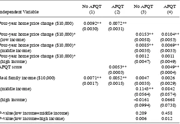
No AFQT (1)
AFQT (2)
No AFQT (3)
AFQT (4)
Four- year home price change ($10,000) 0.0092** 0.0072** (0.0030) (0.0031)
Four- year home price change ($10,000)* 0.0153** 0.0104**
I(low income) (0.0058) (0.0053)
Four- year home price change ($10,000)* 0.0085** 0.0069**
I(middle income) (0.0035) (0.0033)
Four- year home price change ($10,000)* 0.0012 0.0011
I(high income) (0.0047) (0.0049)
AFQT score 0.0053** 0.0049**
(0.0003) (0.0004)
Real family income ($10,000) 0.0071** 0.0052** 0.0047 0.0026 (0.0017) (0.0015) (0.0035) (0.0029)
I(middle income) 0.1143** 0.0842
(0.0564) (0.0574)
I(high income) –0.0161 0.0668
(0.0994) (0.0738)
P- value(low income=middle income) 0.209 0.458
P- value(low income=high income) 0.006 0.012
Notes: All estimates include MSA and age in 1997 fi xed effects as well as controls for mother’s and father’s education, gender, race, MSA- level unemployment and real income per capita, state- level public and private institutions per college age popula-tion, per- student state need- based aid, the ratio of BA to associates degree wages, the ratio of BA to high school wages, and the number of each type of college in each MSA. All estimates also are weighted by NLSY97 sampling weights and include only homeowners. Each row in the table comes from a separate logit model. Housing price changes are real housing price changes over the four years prior to students turning 18 predicted by the conventional mortgage housing price index. Low- income families are those with total income under $75,000, medium income families are those with total income between $75,000 and $125,000, and high- income families are those with total income over $125,000. Standard errors clustered at the MSA- level are in parentheses: ** indicates signifi cance at the 5 percent level and * indicates signifi cance at the 10 percent level.
that the housing boom caused signifi cant changes among lower and middle- income families in the sectors in which their children enrolled in college.
B. Extensive Margin Estimates
The Journal of Human Resources 22
NLSY97 data. In order to explore the importance of controlling for student academic ability, which is not available in the PSID, we estimate the model both with and with-out AFQT scores. In Column 1, we fi nd each $10,000 in housing wealth leads to a 0.0092 percentage point increase in college enrollment. This estimate is very similar to Lovenheim (2011).20 In the next column, we control for AFQT scores and the estimate drops to 0.0072. This result is suggestive of a small upward bias from excluding pre-collegiate ability measures, but the bias is small and Column 2 still points to a positive and statistically signifi cant effect of home price changes on college enrollment.
In Columns 3 and 4, we allow the estimates to vary by household income. Similar to Table 4, we fi nd the lower- income sample to be most responsive to home price changes. A $10,000 increase in home prices is associated with a 0.015 percentage point higher likelihood of attending college, which is statistically different from the highest- income group estimate at the 1 percent level in both columns. The estimates change little when AFQT scores are included. However, these results are smaller than in Lovenheim (2011), who fi nds a marginal effect of 0.0567 for each $10,000 change in home equity. These differences could be due to differences in when income is mea-sured with respect to when students turn 18, differences in the timing of the sample, differences in the samples themselves, or differences in how housing wealth is mea-sured. Despite the fact that the estimates are somewhat smaller for the lower- income sample in Table 5, they still point to a rather large and statistically signifi cant effect of home price changes on college enrollment that is robust to controlling for AFQT scores. This fi nding suggests that while the primary determinant of college attendance may well be student ability (see Carneiro and Heckman (2002) for a discussion), conditional upon that ability there still is a role for short run changes in household resources to affect college attendance.
C. Effects on Applications and Admissions
That housing wealth impacts whether and where students attend college is suggestive that it may impact application behavior. In Table 6, we examine the effects of housing wealth on applications and admissions in order to shed light on some of the mecha-nisms by which housing wealth infl uences college choices. In Panel A, we estimate poisson regressions of the number of applications at four- year institutions by sector, where the control variables are the same as those in Equation 2 in addition to MSA fi xed effects.21 Each column is a separate regression, and we fi nd that each $10,000 increase in home prices leads to a 1 percent increase in applications. The effects are larger for nonfl agship and fl agship applications, at 2.7 and 3.3 percent respectively. Consistent with our fi ndings above, home price changes are uncorrelated with private
20. Note that Lovenheim (2011) estimates instrumental variables models in which four- year home equity changes are used to instrument for contemporaneous home equity. We cannot use this method with the NLSY97 data because we do not have information on home equity changes. He also includes renters in his baseline model.
L
ove
nhe
im
a
nd Re
ynol
ds
23
Table 6
The Effect of Housing Price Changes on Application Decisions and Admission Probabilities
Panel A: Number of Applications
Total Flagship
Non-
fl agship
Four- year Private
Apply to Two- year?
Four- year home price change ($10,000) 0.010** 0.033** 0.027* –0.002 0.004
(0.005) (0.008) (0.014) (0.011) (0.016)
AFQT score 0.006** 0.013** 0.010** 0.015** –0.032**
(0.001) (0.002) (0.002) (0.003) (0.002)
Real family income ($10,000) –0.0001 –0.001 –0.007 0.001 –0.025**
(0.004) (0.007) (0.008) (0.009) (0.012)
Panel B: Number of Admissions
Total Flagship
Non-
fl agship
Four-year Private
Four- year home price change ($10,000) 0.012** 0.037** 0.027 –0.008
(0.005) (0.008) (0.016) (0.014)
AFQT score 0.007** 0.013** 0.012** 0.017**
(0.001) (0.002) (0.002) (0.003)
Real family income ($10,000) –0.003 –0.005 –0.009 0.0003
(0.004) (0.009) (0.009) (0.009)
T
he
J
ourna
l of H
um
an Re
sourc
es
24
Table 6 (continued)
Panel C: Number of Admissions, Conditional on Applying
Total Flagship
Non-
fl agship
Four- year
Private
Four- year home price change ($10,000) 0.012** 0.009 0.018* –0.015
(0.005) (0.011) (0.010) (0.017)
AFQT score 0.007** 0.002 –0.00003 0.005**
(0.001) (0.002) (0.002) (0.002)
Real family income ($10,000) –0.003 –0.005 –0.006 0.009
(0.004) (0.102) (0.007) (0.006)
Lovenheim and Reynolds 25
school applications. The fi nal column in Table 6 shows logit estimates of the effect of home price changes on the likelihood of applying to a two- year school. Even though two- year attendance falls with home price increases, the likelihood of applying to one does not. Thus, students whose families experience home price increases while in high school submit more applications overall and submit more in particular to public four- year schools, including fl agships.
In Panel B, we show the relationship between admissions and home price changes. These estimates include the change in applications shown in Panel A, and they are very similar to those estimates. This similarity suggests the admissions effect is being driven by the applications, not by the relative likelihood of being admitted conditional on applying. Panel C shows these conditional likelihoods, and while the estimates for fl agships and nonfl agships are positive, they are much smaller than the estimates in Panel A. This is particularly true for the fl agship estimates, which indicate that family resource changes while in high school affect applications to more elite public institu-tions that students are qualifi ed to attend. An actual or perceived lack of resources ap-pears to dissuade at least some students from applying to, and thus attending, fl agship state universities. We argue below in Section IV.E that this result is not being driven by changes in investments during high school or in high school quality. Rather, the evidence points to family resources when students are in high school directly affect-ing application and attendance decisions of students in a manner that affects higher education quality.
D. Direct Resource and Quality Effects
Because college sector is an imperfect proxy for college resources and because stu-dents may be changing their selection behavior within our four sectors when home prices change, we examine the effect of housing price changes on direct quality and resource measures in Table 7. In the table, each cell for the full sample results comes from a separate regression of Equation 3, and for the results by income, each row comes from a separate regression.
The estimates suggest that students attend higher quality and resource institutions when their parents’ home value increases over the previous four years. For example, a $10,000 increase in four- year home prices increases the 75th percentile SAT scores of the attending university by 0.80 points, the student- faculty ratio by 0.0003, expen-ditures per student by $289.92, instructional expenexpen-ditures per student by $63.60, and the six- year BA graduation rate of the university by 0.001. Although many of these marginal effects are modest, each of these measures is at best a partial proxy for the underlying quality of the institution. Furthermore, when multiplied by the average changes in home prices shown in Table 2, these marginal effects translate into sizeable institutional quality changes experienced by students, which are driven by changing enrollment decisions. Table 7 also shows that home price changes have at most a small effect on posted tuition.22 Given that most students are likely to receive federal, state, and institutional aid, however, posted tuition may be a poor measure of the amount actually paid by families.
The Journal of Human Resources 26
The remaining columns in Table 7 present estimates that vary by income group. As with the multinomial logit results, the effects are largest for the lowest- income group. All estimates except for tuition are positive and are statistically signifi cantly different from zero at the 5 or 10 percent level. Although students from both lower and middle- income families attend institutions with higher SAT scores and with higher graduation rates when home prices increase, there is no signifi cant effect among families with income greater than $125,000 per year. The multinomial logit estimates are suggestive that at least some of these results are being driven by the higher likelihood of both lower and middle income families to send their children to fl agship public schools that have higher resources when they experience housing price increases.
Table 7
OLS Estimates of the Effect of Housing Price Changes on College Resources
Independent Variable:
Faculty- student ratio 0.0003** 0.0004** 0.0002 0.0002 (0.0001) (0.0002) (0.0002) (0.0002)
Lovenheim and Reynolds 27
E. Robustness Checks
Interpreting the estimates in Tables 3–7 as causal relies on several assumptions about the exogeneity of home price changes that were discussed in Section III. In this sec-tion, we show a series of robustness checks in order to assess the sensitivity of our results to many of these assumptions. In Column 1 of Table 8, we show estimates from Equations 2 and 3 using only renters.23 We assign each renter the four- year percent-age change in the CMHPI for his MSA. These regressions are informative because they check whether unobserved factors at the MSA level, such as high- skilled labor demand, are affecting both home prices and college selection for all residents. Further-more, these estimates show whether it is appropriate to restrict our main analysis to home owners. Table 8 presents evidence that renters do not alter their school choices in response to MSA- level home price changes. In neither panel is any estimate statisti-cally different from zero at conventional levels, and the estimates are universally small in magnitude.
The estimates for renters suggest that our results are not being driven by home price changes infl uencing K- 12 education quality, as such quality changes would be experienced by both renters and home owners. In order to explore this issue further, we examine whether four- year home price changes while in high school impact the likelihood of attending a private school, the size of one’s high school, teacher- student ratios, high school GPA, the number of AP tests taken, and hours worked while in high school. We also investigated the impact of housing price changes on the likeli-hood of high school completion in the full sample. In no case is there a statistically or economically signifi cant relationship between home price changes and these variables, which suggests our estimates are not being driven by differential investment in human capital while in high school. All results are available upon request.
In Column 2 of Table 8, we control for 1997 home prices. These estimates dis-tinguish between the effects of owning an expensive home and the effect of being exposed to home price changes based on one’s location and age. The results in both columns are qualitatively and quantitatively similar to those in Tables 3 and 7. Overall, the estimates indicate that MSA- level home price changes are the main driver of our results, which supports many of our identifi cation assumptions because this source is the most likely to be exogenous.24
Throughout much of this analysis, we have excluded nonattenders from the sample in order to make the multinomial logit and the school resource samples the same. However, as shown in Table 5 and in Lovenheim (2011), the extensive margin also is affected by home price changes. In Column 3, Panel A of Table 8, we include nonat-tendance as its own category in our multinomial logit model. The marginal effects are very similar to those in Table 3, which suggests the exclusion of this group is not driving our results and conclusions.
Furthermore, our categorization of college sectors may be problematic because
23. Descriptive statistics by 1997 home owner status are presented in Online Appendix Table A- 2. 24. We also have controlled for four- year home price growth when students are between 21 and 24, and we
The Journal of Human Resources
Flagship / top 50 public 2.52e–9 0.0023** 0.0014** 0.0024* (3.90e–9) (0.0011) (0.0005) (0.0014)
Four- year private 0.0002 –0.0014 0.0012 0.0001
(0.0002) (0.0028) (0.0016) (0.0018)
Faculty- student ratio 0.0003 0.0003** 0.0003** 0.0002* (0.0002) (0.0001) (0.0001) (0.0001)