ANALYSIS OF
PAVEMENT
STRUCTURES
Animesh Das
Professor, Department of Civil Engineering Indian Institute of Technology Kanpur
© 2015 by Taylor & Francis Group, LLC
CRC Press is an imprint of Taylor & Francis Group, an Informa business
No claim to original U.S. Government works Version Date: 20140617
International Standard Book Number-13: 978-1-4665-5856-4 (eBook - PDF)
This book contains information obtained from authentic and highly regarded sources. Reasonable efforts have been made to publish reliable data and information, but the author and publisher cannot assume responsibility for the validity of all materials or the consequences of their use. The authors and publishers have attempted to trace the copyright holders of all material reproduced in this publication and apologize to copyright holders if permission to publish in this form has not been obtained. If any copyright material has not been acknowledged please write and let us know so we may rectify in any future reprint.
Except as permitted under U.S. Copyright Law, no part of this book may be reprinted, reproduced, transmit-ted, or utilized in any form by any electronic, mechanical, or other means, now known or hereafter inventransmit-ted, including photocopying, microfilming, and recording, or in any information storage or retrieval system, without written permission from the publishers.
For permission to photocopy or use material electronically from this work, please access www.copyright. com (http://www.copyright.com/) or contact the Copyright Clearance Center, Inc. (CCC), 222 Rosewood Drive, Danvers, MA 01923, 978-750-8400. CCC is a not-for-profit organization that provides licenses and registration for a variety of users. For organizations that have been granted a photocopy license by the CCC, a separate system of payment has been arranged.
Trademark Notice: Product or corporate names may be trademarks or registered trademarks, and are used only for identification and explanation without intent to infringe.
List of Symbols xiii
List of Figures xvii
Preface xxiii
About the Author xxvii
1 Introduction 1
1.1 Purpose of the book . . . 1
1.2 Background and sign conventions . . . 4
1.2.1 State of stress . . . 5
1.2.2 Strain-displacement and strain
compatibility equations . . . 9
1.2.3 Constitutive relationship between stress and strain . . . 11
1.2.4 Equilibrium equations . . . 14
1.3 Closure . . . 15
2 Material characterization 17
2.1 Introduction . . . 17
2.2 Soil and unbound granular material . . . 17
2.3 Asphalt mix . . . 20
2.3.1 Rheological models for asphalt mix . . . 21
2.3.2 Fatigue characterization . . . 42
2.4 Cement concrete and cemented material . . . 44
2.5 Closure . . . 45
3 Load stress in concrete pavement 47 3.1 Introduction . . . 47
3.2 Analysis of beam resting on elastic foundation . . . 47
3.2.1 Beam resting on a Winkler foundation . . . 53
3.2.2 Beam resting on a Kerr foundation . . . 55
3.2.3 Various other models . . . 57
3.3 Analysis of a thin plate resting on an elastic foundation . . . 58
3.3.1 Plate resting on a Winkler foundation . . . 58
3.3.2 Plate resting on a Pasternak foundation . . 64
3.3.3 Plate resting on a Kerr foundation . . . 65
3.3.4 Boundary conditions . . . 66
3.4 Load stress in a concrete pavement slab . . . 67
4 Temperature stress in concrete pavement 73
4.1 Introduction . . . 73
4.2 Thermal profile . . . 73
4.2.1 Surface boundary conditions . . . 75
4.2.2 Interface condition . . . 76
4.2.3 Condition at infinite depth . . . 76
4.3 Thermal stress in concrete pavement . . . 77
4.3.1 Thermal stress under a fully restrained condition . . . 77
4.3.2 Thermal stress under a partially restrained condition . . . 84
4.4 Closure . . . 90
5 Load stress in asphalt pavement 91 5.1 Introduction . . . 91
5.2 General formulation . . . 91
5.3 Solution for elastic half-space . . . 95
5.4 Multi-layered structure . . . 103
5.4.1 Formulation . . . 104
5.4.2 Boundary conditions . . . 107
5.4.3 Discussions . . . 109
5.5 Closure . . . 112
6.2 Thermal profile . . . 116
6.3 Thermal stress in asphalt pavement . . . 116
6.4 Closure . . . 119
7 Pavement design 121 7.1 Introduction . . . 121
7.2 Design philosophy . . . 122
7.3 Design parameters . . . 127
7.3.1 Material parameters . . . 127
7.3.2 Traffic parameters and design period . . . . 127
7.3.3 Environmental parameters . . . 127
7.4 Design process . . . 128
7.4.1 Thickness design . . . 128
7.4.2 Design of joints . . . 134
7.4.3 Estimation of joint spacing . . . 134
7.4.4 Design of dowel bar . . . 136
7.4.5 Design of tie bar . . . 137
7.5 Maintenance strategy . . . 138
7.6 Closure . . . 141
8 Miscellaneous topics 143 8.1 Introduction . . . 143
8.3 Plates/beams resting on an elastic foundation
subjected to dynamic loading . . . 146
8.4 Analysis of composite pavements . . . 149
8.5 Reliability issues in pavement design . . . 150
8.6 Inverse problem in pavement engineering . . . 152
8.7 Closure . . . 154
References 157
a Radius of circular area or equivalent tire imprint
A Area
ast Cross-sectional area of a single steel bar Ast Cross-sectional area of steel per unit length B Width of a concrete slab
BF Body force
Ccrp Creep compliance Ch Heat capacity
D Flexural rigidity of a plate
E Young’s modulus or elastic modulus
E′ Storage modulus
E′′ Loss modulus
E∗ Complex modulus
Ed Dynamic modulus Erel Relaxation modulus f Coefficient of friction
g Acceleration due to gravity
G Shear modulus
h Layer thickness
I1 First stress invariant (=σ1+σ2+σ3)
I2 Second stress invariant
I3 Third stress invariant
k Modulus of subgrade reaction
ktd Coefficient of thermal diffusivity ks Spring constant
kss Slider constant
l Radius of relative stiffness
L Length of a concrete slab
M Moment
MR Resilient modulus
Mc Unit cost of maintenance Mu Unit road user cost
n Number of repetitions applied
N Number of traffic repetitions a material/pavement can
sustain
Pa Atmospheric pressure q Pressure
Q Concentrated load
Qh Heat flow per unit area r Discount rate
R Reliability
S Structural health of a pavement
t Time
T Temperature
T Number of expected traffic repetitions
Tt Temperature at the top surface Tb Temperature at the bottom surface T∞ Temperature at infinite depth
u Displacement along X direction (Cartesian coordinate)
ur Displacement along R direction (cylindrical coordinate) U Universal gas constant
v Displacement along Y direction (Cartesian coordinate)
V Shear force
vθ Displacement along tangential direction (cylindrical
co-ordinate)
Vo Speed
x Distance along X direction
y Distance along Y direction
z Distance along Z direction
zs Gap between two adjacent concrete slabs α Coefficient of thermal expansion
αT Time shift factor β An angle
δ Phase angle
∆H Apparent activation energy
ǫ Strain
ζ Dummy variable for time
θ An angle in cylindrical polar coordinate system
ηd Viscosity of the dashpot µ Poisson’s ratio
ρ Density of the material
σ Normal stress
σc Confining pressure (=σ3) σd Deviatoric stress
σS Tensile strength
σT A Axial stress component due to temperature σT B Bending stress component due to temperature σT N Nonlinear stress component due to temperature
ω Displacement along Z direction (for both Cartesian and cylindrical coordinates)
1.1 Typical cross-section of an asphalt and a concrete pavement. . . 2
1.2 Dowel bar and tie bar arrangement in concrete pavement. . . 2
1.3 Sign convention in the Cartesian system followed in this book. . . 5
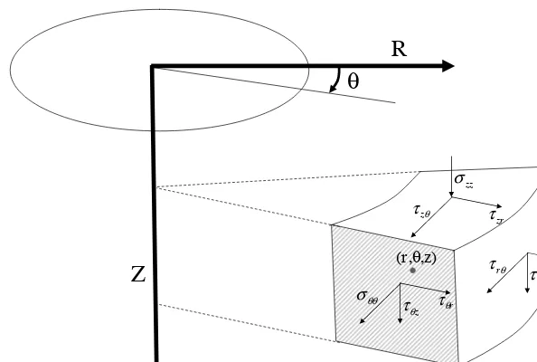
1.4 Sign convention in the cylindrical system followed in this book. . . 6
1.5 Stresses on plane “afh” plane with direction cosines as l, m and n. . . 7
2.1 Soil and unbound granular materials are used for building roads. . . 18
2.2 Repetitive load is applied to unbound granular ma-terial (or soil) in a triaxial setup to estimate MR
value. . . 18
2.3 Cross-sectional image of an asphalt mix sample. . . 21
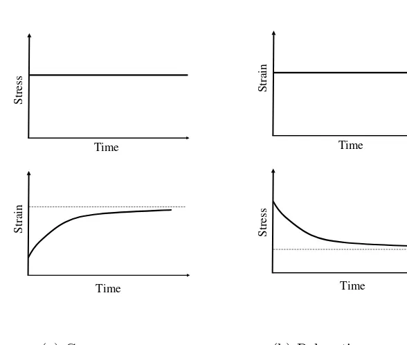
2.4 Typical creep and relaxation response of asphalt mix. 22
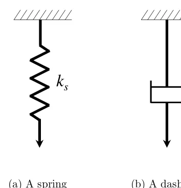
2.5 A spring and a dashpot. . . 23
2.6 A Maxwell model. . . 24
2.7 A Kelvin–Voigt model. . . 26
2.8 A three-component model. . . 27
2.9 Sinusoidal loading on rheological material in stress controlled mode. . . 28
2.10 A generalized Maxwell model. . . 31
2.11 A generalized Kelvin model. . . 31
2.12 A strain-controlled thought experiment. . . 33
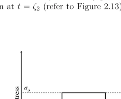
2.13 A stress of magnitude σo applied at t = ζ1 on a rheologic material, then withdrawn at t=ζ2. . . 35
2.14 Strain response of Kelvin–Voigt model with a stress of magnitude σo applied at t = ζ1 and then with-drawn at t=ζ2. . . 37
2.15 A stress of magnitudeσois applied linearly byt=ζ1 to a rheologic material. . . 37
2.16 Schematic diagram illustrating the principle of time–temperature superposition. . . 40
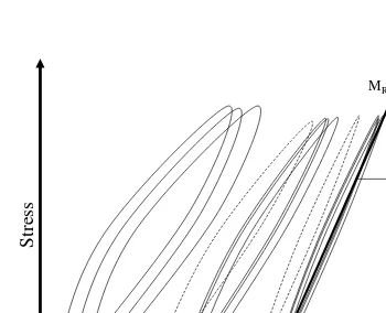
2.17 Schematic diagram showing a possible fatigue be-havior of bound materials in simple flexural fatigue testing. . . 43
3.1 A beam resting on numerous springs is acted on by a concentrated load Q. . . 48
3.2 Free-body diagram of dx elemental length of the beam presented in Figure 3.1. . . 49
3.5 A beam with an arbitrary loading. . . 52
3.6 A beam resting on a Pasternak foundation and a free-body-diagram of the shear layer. . . 54
3.7 A beam resting on a Kerr foundation and a free-body diagram of the shear layer. . . 56
3.8 Deflected position of an element of a thin plate. . . 59
3.9 Free-body diagram of an element of a thin plate. . . 62
3.10 Free-body diagram of the shear layer of a two-dimensional Pasternak foundation. . . 64
3.11 The slab boundaries may be free, fixed, or hinged. . 66
3.12 A slab resting on a Winkler spring acted upon by a rectangular patch loading. . . 68
3.13 Schematic diagram showing variation of bending stress (due to load at interior) with slab thickness and modulus of subgrade reaction. . . 71
4.1 Schematic diagram showing one-dimensional steady-state heat flow across a medium. . . 74
4.2 A one-dimensional schematic representation of de-velopment of thermal stress in concrete slab. . . 78
4.3 The thermal profile and thermal stress components for the example problem (when Tt> Tb). . . 83
4.4 Schematic diagram showing variation σT B for T t> Tb when (i) fully restrained and (ii) finite restraint
is provided by self-weight. . . 84
4.6 Free-body diagram of an element of length dx and width B of the slab. . . 86
4.7 Slab resting on spring sliders. . . 87
4.8 A schematic diagram representing the variation of
σxx andualong the length of the slab for the partial
restraint condition in the model shown in Figure 4.7. 88
5.1 A point load acting vertically on a half-space. . . . 95
5.2 Circular loading on an elastic half-space. . . 99
5.3 Displacement of an elastic half-space due to a flex-ible uniformly loaded circular plate. . . 100
5.4 Displacement of an elastic half-space due to a rigid circular plate . . . 102
5.5 A multi-layered asphalt pavement structure. . . 104
5.6 Typical output from an analysis of a multi-layered elastic structure. . . 110
5.7 A typical tire imprint. . . 111
5.8 Shear stress acting within a circular area of
radius a. . . 112
5.9 Superposition may be assumed for computing re-sponse due to multi-axle loading. . . 113
6.1 A conceptual diagram of the variation of thermal stress (σT(t)) with temperature (T) and time (t). . 117
7.1 Schematic diagram representing two possible mech-anisms of rutting. . . 125
7.2 A schematic diagram indicating the possible rel-ative magnitudes (not to scale) and nature (ten-sion/compression) of load and thermal bending stresses in concrete pavement at the corner, edge, and interior. . . 129
7.3 A generic pavement design scheme, where thick-nesses are decided based on critical
stresses/strains. . . 129
7.4 A generic pavement design scheme where thick-nesses are decided based on the number of
repetitions. . . 131
7.5 Schematic diagram explaining the thermal expan-sion joint spacing. . . 135
7.6 Schematic diagram of a single tie bar. . . 137
7.7 Schematic diagram showing variation of structural health of pavement over maintenance cycles. . . 139
8.1 An infinite beam resting on an elastic half-space. . 144
8.2 An infinite beam subjected to a moving dynamic
load. . . 147
8.3 Estimation of reliability from distributions of N
and T. . . 151
8.4 Schematic diagram of pavement design chart. . . . 152
This is a simple book.
This book is about pavement analysis. A pavement is a multi-layered structure, made of a number of layers placed one over the other. These layers can be made of asphaltic material, cement concrete, bound or unbound stone aggregates, etc. These materials show complex mechanical response with the variation of stress, time, or temperature. Thus, understanding the performance of an in-service pavement structure subjected to vehicular loading and environmental variations is a difficult task.
However, this is a simple book. This book presents a step-by-step formulation for analyses of load and thermal stresses of ideal-ized pavement structures. Some of these idealizations involve as-sumptions of the material being linear, elastic, homogeneous and isotropic; the load being static; the thermal profile being linear and so on.
Significant research has been done on analysis and design of pave-ments during the last half-century (some of the fundamental devel-opments are, however, more than hundred years old) and a large number of research publications are already available. However, there is a need for the basic formulations to be systematically compiled and put together in one place. Hence this book. It is believed that such a compilation will provide an exposure to the basic approaches used in pavement analyses and subsequently help
the readers formulate their own research or field problems—more difficult than those dealt with in this book.
The idea of this book originated when I initiated a post-graduate course on Characterization of Pavement Materials and Analysis of Pavements at IIT Kanpur. This course was introduced in 2007; that was the time we were revising the post-graduate course struc-ture in our department. I must thank my colleague Dr. Partha Chakroborty for suggesting at that time that the Transportation Engineering program at IIT Kanpur should have a pavement en-gineering course with more analysis content. I also should thank him for his constant encouragement during the entire process of preparing this manuscript. One of our graduate students, Priyanka Khan, typed out portions of my lectures as class-notes. Those ini-tial pages helped me to overcome the inertia of getting started to write this book. That is how it began.
Since this book provides an overview of basic approaches for pave-ment analysis, rigorous derivations for complex situations have been deliberately skipped. However, references are provided in appropriate contexts for readers who want to explore further. I must place a disclaimer that those references are not necessarily the only and the best reading material, but they are just a repre-sentative few.
A number of my former and present students have contributed to the development of this book. They have asked me questions inside the classroom and outside. Discussions with some of them were quite useful, while others helped me to cross-check a few deriva-tions. Dr. Pabitra Rajbongshi, Sudhir N. Varma, Vivek Agarwal, Pranamesh Chakraborty, Syed Abu Rehan, and Vishal Katariya are some of these students. I must also thank my former colleague, Dr. Ashwini Kumar, for the useful discussions with him on plate theories. I also thank all the people with whom I have interacted professionally from time to time for discussing various issues re-lated to pavement engineering. I want to thank all the authors of numerous papers, books and other documents whose works have been referred to in this book.
I am most grateful to my parents for their care and thought in-volved in my education. I thank my father, Dr. Kali Charan Das, for teaching me formulations in physics using first principles. I thank my Ph.D. supervisor Dr. B. B. Pandey for training me as a researcher in pavement engineering. I also wish to thank my col-leagues for the encouragement, and my Institute, IIT Kanpur, for providing an excellent academic ambiance.
Care has been taken as far as possible to check for editorial mis-takes. If, however, you find any, or wish to provide your feedback on this book please drop me an e-mail at [email protected].
This book now must go for printing.
Animesh Das, Ph.D., is presently working as a professor in the Department of Civil Engineering, Indian Institute of Technology Kanpur. He earned his Ph.D. degree from the Indian Institute of Technology Kharagpur. Dr. Das’s areas of interest are pavement material characterization, analysis, pavement design, and pave-ment maintenance. He has authored many technical publications in various journals of repute and in conference proceedings. He has co-authored a textbook titled Principles of Transportation Engi-neeringpublished by Prentice-Hall of India (currently, PHI Learn-ing), and he co-developed a web-course titled Advanced Trans-portation Engineeringunder the National Programme on Technol-ogy Enhanced Learning (NPTEL), India. Dr. Das has received a number of awards in recognition of his contribution in the field, in-cluding an Indian National Academy of Engineers Young Engineer award (2004) and a Fulbright–Nehru Senior Research Fellowship (2012–13), etc. Details of his works can be found on his webpage: http://home.iitk.ac.in/∼adas.
Introduction
1.1
Purpose of the book
Pavement is a multi-layered structure. It is made up of compacted soil, unbound granular material (stone aggregates), asphalt mix or cement concrete (or other bound material) put as horizontal layers one above the other. Figure 1.1 presents a typical cross section of an asphalt and a concrete pavement.
Generally, asphalt pavements do not have joints, whereas the con-crete pavements (commonly known as jointed plain concon-crete pave-ment) have joints1. The concrete pavements are made of concrete
slabs of finite dimensions with connections (generally of steels bars) to the adjacent slabs. Dowel bars are provided along the transverse joint and tie bars are provided along the longitudinal joint (refer to Figure 1.2). A block pavement or a segmental pave-ment is made up of inter-connected blocks (generally, cepave-ment con-crete blocks), and its structural behavior is different from the usual asphalt or concrete pavements.
1
Though exceptions are possible, for example, asphalt pavements in ex-tremely cold climates may be provided with joints, continuously reinforced concrete pavements does not generally have joints etc.
Subgrade (soil)
Subbase course (cound/ unbound granular)
Base course (bound/ unbound granular)
Binder course (bituminous)
Wearing course (bituminous)
(a) An asphalt pavement section
Concrete slab
Base course (lean cement concrete/ roller compacted concrete)
Subgrade (soil)
(b) A concrete pavement section
Figure 1.1: Typical cross-section of an asphalt and a concrete pave-ment.
dow
el bars tie bar
s
An in-service pavement is continuously subjected to traffic load-ing and temperature variations. The purpose of this book is to present a conceptual framework on the basic formulation of load and thermal stresses of typical (as shown in Figures 1.1 and 1.2) concrete and asphalt pavements.
Analysis of pavement structure enables one to predict or explain the pavement response to load from physical understanding of the governing principles, which can be corroborated later through ex-perimental observations. This, in turn, builds confidence in struc-tural design, evaluation, and maintenance planning of road infras-tructure.
Generally speaking, a concrete pavement is idealized as a plate resting on an elastic foundation [124, 303, 304, 305]. It is assumed that the load is transferred through bending and the slab thickness does not undergo any change while it is subjected to a load. For an asphalt pavement, it is assumed that the load is transferred through contacts of particles, and the layer thicknesses do undergo changes due to application of load [34, 35, 142].
Pavement being a multi-layered structure, it is generally difficult to obtain a closed-form solution of its response due to load. For design purpose, pavement analysis may be done through some software(s) which may use certain numerical methods to perform the analysis. Ready-to-use analysis charts are also available in various codes/ guidelines. The algorithms used and the assumptions involved in the analysis process may not always be apparent to a pavement designer (as a user of these softwares/charts). Thus, there is a need to know the assumptions involved and the basic formulations needed for analyzing a pavement structure.
basic formulations might have been developed many years ago (of-ten with different notations and sign conventions than practiced today) and contributed by researchers from other areas of science and engineering. For instance, contributions to the theoretical for-mulation for pavement analysis have come from structural engi-neering (for example, the theory of plates), soil mechanics (for example, beams and plates on an elastic foundation), applied me-chanics (for example, the stress-strain relationship, principles of rheology), mechanical engineering (for example, material model-ing) and so on.
For a beginner (in pavement engineering) this may appear to be a hurdle—because, one may need to trace back to the original source, understand the assumptions/idealizations, and follow the subsequent theoretical development. Thus, there is a need for the approaches to pavement analyses to be collated in one place. This is the purpose of this book. The focus of the present book, there-fore, can be identified as follows,
• This book is a compilation of the existing knowledge on anal-yses of pavement structure. Load and thermal stress analanal-yses for both asphalt and concrete pavements are dealt with in this book. Attempts have been made to provide ready refer-ences to other publications/documents for further reading.
• Basic formulations for analysis of pavement structure have been presented in this book in a step-by-step manner—from a simple formulation to a more complex one. Attempts have been made to maintain a uniformity in symbol and sign con-ventions throughout the book.
1.2
Background and sign conventions
X
Figure 1.3: Sign convention in the Cartesian system followed in this book.
and the theory of elasticity [11, 99, 241, 277] for further study; applications of some of these formulations can also be found in books on soil mechanics [63, 104, 162, 222]. The sign convention followed in the present book is shown in Figure 1.3 for the Carte-sian coordinate system and in Figure 1.4 for the cylindrical coordi-nate system. These figures also show the notations used to identify the stresses in different directions.
1.2.1
State of stress
The state of stress in a Cartesian coordinate system (refer to Fig-ure 1.3) can be written as,
R
Figure 1.4: Sign convention in the cylindrical system followed in this book.
σ is also known as Cauchy’s stress. For normal stresses on a body,
a negative sign has been used in this book to indicate compression, and a positive sign to indicate tension.
Figure 1.5 shows a plane “afh,” whose direction cosine values are
l, m and n with respect to X, Y and Z axes respectively. If, psx, psy and psz represent the stresses (on plane “afh”) parallel to X,
Y and Z (refer Figure 1.5(a)), then,
The normal stress in the plane “afh” (refer to Figure 1.5b) can be obtained as,
σs =psxl+psym+pszn (1.3)
The shear stress on plane “afh” is obtained as,
τs= p2sx+p2sy+p2sz
−σs21/2
X
Figure 1.5: Stresses on plane “afh” plane with direction cosines as
l, m and n.
For a special case, when the choice of the plane “afh” (that is choice of l, m and n) is such that the shear stress vanishes, and therefore, only the normal stress exists (that is, principal stress on that plane), it can be written as,
For a feasible solution to exist,
The Equation 1.6 gives rise to the characteristic equation as,
where,I1,I2andI3are coefficients. Since the principal stress value for a given state of stress should not vary with the choice of the reference coordinate axes, the coefficients I1, I2 and I3 must have constant values. These are known as stress invariants. Their ex-pressions are provided as Equations 1.8–1.10.
I1 =σxx+σyy+σzz (1.8)
I2 =σxxσyy+σyyσzz +σzzσxx−τxy2 −τyz2 −τzx2 (1.9)
I3 =σxxσyyσzz + 2τxyτyzτzx−σxxτyz2 −σyyτxz2 −σzzτxy2 (1.10)
In terms of principal stresses, these take the following form,
I1 =σ1+σ2+σ3 (1.11)
I2 =σ1σ2+σ2σ3+σ3σ1 (1.12)
I3 =σ1σ2σ3 (1.13)
There can be a special case when l, m, n values are all equal with references to the principal axes. That is, l = m = n = √1
3.
The corresponding plane is known as an octahedral plane. The octahedral normal stress (σoct) can be obtained from Equation 1.3
as follows,
σoct =
1
3(σ1+σ2+σ3) (1.14)
The octahedral shear stress (τoct) can be obtained from
Equa-tion 1.4 as follows,
τoct =
1
3 (σ1−σ2)
2+ (σ1−σ3)2+ (σ3−σ1)21/2
The σoct and τoct in terms of the general state of stress can be
1.2.2
Strain-displacement and strain
compatibility equations
If displacement fields in the direction of X, Y and Z are considered as u, v, and ω then,
Z directions) and γxy, γyz and γzx indicate the engineering shear
strains. By taking partial derivatives and suitably substituting, one can develop the following set of equations which do not contain the
as strain compatibility equations.
The strain-displacement relationships in the cylindrical coordinate are,
where, ur = displacement inr direction, vθ = displacement along
1.2.3
Constitutive relationship between stress
and strain
The constitutive relationship for a linear anisotropic material can be written as,
C21 C22 C23 C24 C25 C26
C31 C32 C33 C34 C35 C36
C41 C42 C43 C44 C45 C46
C51 C52 C53 C54 C55 C56
C61 C62 C63 C64 C65 C66
where,Cij are the material constants. For isotropic material (that
is, when the properties are same along any direction) Equation 1.21 takes the following form:
modulus of the material. The inverted form of the Equation 1.22 can be presented (using the values of C11 and C12) as following,
Equation 1.23 can be written as,
2(1+µ). In a cylindrical coordinate (for isotropic
mate-rial), the equations are,
σrr =
Plane stress condition (in Cartesian coordinate system)
For a plane stress condition, stress in one particular direction (say along Y direction) is zero. That is, σyy = σxy = σyz = 0. Such
a situation arises, for example, for a disk with a negligible thick-ness. Putting these conditions in Equations 1.24 and 1.25, one can write,
Conversely, the stresses (in the plane stress case) can be expressed (considering, G= E
2(1+µ)) in terms of strains as follows,
Plane strain condition in (Cartesian coordinate system)
In a plane strain condition, strain in one particular direction (say along Y direction) is zero. That is,ǫyy =γxy =γyz = 0. Such a
strain along the longitudinal direction. Putting these conditions in Equations 1.24 and 1.25, one can write,
ǫxx =
Conversely, the stresses (in the plane strain case) can be expressed in terms of strains as follows,
σxx =
The equilibrium condition is derived by taking the force balance along each direction. The static equilibrium equation (in Cartesian coordinate system) can be written as,
∂σxx
directions respectively. For a dynamic equilibrium case, the right-hand side of the equations will have terms asρ∂2u
∂t2,ρ∂ 2v
∂t2 and ρ∂ 2ω
∂t2,
respectively, whereρis the density of the material. The static equi-librium condition in a cylindrical coordinate system is obtained as,
∂σrr
along r, θ, and Z directions respectively.
1.3
Closure
Material characterization
2.1
Introduction
As mentioned in Section 1.1, different materials are used to build a road. This chapter deals with the material characterization of some of the basic types of materials used in pavements. Material characterization for soil, unbound granular material, asphalt mix, cement concrete, and cemented material will be briefly discussed in this chapter.
2.2
Soil and unbound granular
material
Compacted soil is used to build subgrade (refer Figure 2.1(a)). Unbound granular material is used to build the base/sub-base of a pavement structure (refer Figure 2.1(b)).
The resilient modulus (MR) is generally the elastic modulus
pa-rameter used for the characterization of granular material (or soil). It is determined by applying a repetitive load to the sample in a
(a) Compacted soil used as sub-grade
(b) Unbound granular material can be used as a base/sub-base
Figure 2.1: Soil and unbound granular materials are used for build-ing roads.
Strain
S
tr
e
ss
MR
triaxial cell [3]. The MR is defined as,
MR =
deviatoric stress
recoverable strain (2.1)
Experimental studies indicate granular material is a stress depen-dent material. A large number of MR models (as functions of the
state of stress) have been proposed by past researchers. One can refer to, for example, [163, 167, 278, 288] etc., for brief reviews on the various models of granular material and soil. One of such models is [75, 110],
MR =c1(σc/Pa)c2 (2.2)
where, σc is the confining pressure (= σ3) in a triaxial test, P a is
the atmospheric pressure, c1 and c2 are the material parameters.
σc is divided byP
a to make the parameter dimensionless. Another
model, popularly known ask−θ model (θ =I1), is represented as follows [1, 32, 110, 205]
MR =k1(I1)k2 (2.3)
where, k1 and k2 are the material parameters and I1 is the first
invariant of stress (refer to Equations 1.8 and 1.11). It was argued that the model represented by Equation 2.3 has certain limita-tions [163], and the following models were proposed [195, 293]
MR =k1(I1)k2(σd)k3 (2.4)
where, k1, k2 and k2 are the material parameters,σd = deviatoric
stress.
MR =k1(I1)k2(τoct)k3 (2.5)
where, τoct is the octahedral shear stress (refer to Equation 1.15),
and so on.
stress level, etc. Further behavior of granular material in compres-sion and in tencompres-sion (because granular material can only sustain a small magnitude of tension) is different; therefore these need to be modeled separately [318]. It also behaves anisotropically [250]. One can, for example, refer to [163, 278] for a brief review on this topic.
Besides the above kind of models for MR (where, MR values are
related to various stress parameters), a number of other (constitu-tive relationship based) models also have been proposed, in which volumetric and shear strains are considered [26, 29, 30, 160]. In these models, the material (that is, granular material or soil) is assumed to behave as an isotropic (refer Equation 1.22) and non-linearly elastic material, (hence, there will be no loss in the strain energy) or the volumetric strain is path independent.
There are various other parameters which are used to character-ize soil and granular materials, and some of these are related to MR through empirical equations. Modulus of subgrade
reac-tion [1, 217, 281] (k) is another parameter which is measured in situ, typically by a plate load test [102]. This is defined as the pressure needed to cause unit displacement of the plate. This con-ceptually represents the “spring constant” of the foundation on which the pavement is resting. The parameter k will be briefly discussed later in Section 3.2.1.
2.3
Asphalt mix
Figure 2.3: Cross-sectional image of an asphalt mix sample.
Various stiffness modulus parameters, measurement techniques, and modeling have been proposed to characterize asphalt mix [4, 70, 149, 172, 268, 291, 314]. Some of the simple rheological models and associated principles, which can be used to develop simple models for an asphalt mix, are discussed briefly in the following.
2.3.1
Rheological models for asphalt mix
Rheolgical models are widely used to describe the mechanical re-sponse of materials which varies with time. For a detailed un-derstanding on rheological principles one can refer to, for exam-ple, [51, 84, 161] etc. A number of textbooks and synthesis docu-ments are available on rheological modeling of materials.
Time Time
Str
es
s
Str
ai
n
(a) Creep response
Time Time
Str
es
s
Str
ai
n
(b) Relaxation response
Figure 2.4: Typical creep and relaxation response of asphalt mix.
(until it stabilizes to an almost constant level). A typical behavior, observed for asphalt mix, under creep and relaxation conditions is shown in Figures 2.4(a) and 2.4(b) respectively. Various curve fitting techniques (for example, power law, Prony series, etc.) have been suggested to fit the data, and the readers can, for example, refer to [149, 214] for further reading.
Creep modulus (Ecrp) at any given time t can be defined as the
stress divided by the strain at that time under creep condition, and the Creep compliance (Ccrp) at any time t is defined as the
strain divided by the stress at that time under creep condition. Similarly, the relaxation modulus (Erel) at any given time t is
defined as the stress divided by the strain at that time, under relaxation condition.
k
s(a) A spring
η
d(b) A dashpot
Figure 2.5: A spring and a dashpot.
combinations. The constitutive relationship of a (Hookean) spring (refer to Figure 2.5(a)) can be represented as,
σ =ksǫ (2.6)
where, σ = stress in the spring, ks = spring constant, and ǫ =
strain in the spring. The constitutive relationship of a dashpot (refer to Figure 2.5(b)) can be represented as,
σ =ηdǫ˙ (2.7)
where, σ = stress in the dashpot, ηd = viscosity of the dashpot,
and ˙ǫ= strain rate of the dashpot. Various combinations of spring and dashpot are used to develop various models. Since these mod-els are made with elastic (that is, spring) and viscous (that is, dashpot) components, they are expected to capture the viscoelas-tic rheologic behavior of the material.
Two component models
ks
ηd
Figure 2.6: A Maxwell model.
Maxwell model
A Maxwell model is presented in Figure 2.6. Since, in this model, the spring and the dashpot are connected in series, the stresses are equal in each component and the total strain is equal to the sum of the strains in each of the components. Considering these two conditions, the constitutive equation can be written as,
σ+ ˙σηs ks
=ηdǫ˙ (2.8)
where, σ = stress in the system and ǫ= strain in the system. For a creep case, the condition is σ= constant = σo (say), or ˙σ = 0.
The Equation 2.8, therefore, takes the form
σo =ηsǫ˙ (2.9)
Using the condition that at t = 0, ǫ = σo
ηd, the solution of
Equa-tion 2.9 can be obtained as,
ǫ(t) = σo
ηd
t+σo
ks
(2.10)
proposed in Figure 2.4(a). The creep compliance in this case can
For the relaxation case, the condition is ǫ= constant = ǫo (say),
or, ˙ǫ= 0. Equation 2.8 takes the form
σ+ ˙σηd ks
= 0 (2.12)
Using the condition that at t = 0, σ=ksǫo, the solution of
Equa-tion 2.12 can be obtained as,
σ =ksǫoe− kst
ηd (2.13)
The relaxation modulus, therefore, is obtained as,
Erel(t) =σ(t)/ǫo
=kse− ks
ηdt (2.14)
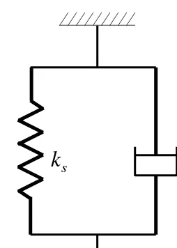
Kelvin–Voigt model
A Kelvin–Voigt model is presented in Figure 2.7. Since, in this model, the spring and the dashpot are connected in parallel, the strains are equal in each component and the total stress is equal to the sum of the stresses in each of the components. Taking these two conditions into account, the constitutive equation can be written as,
σ =ksǫ+ηdǫ˙ (2.15)
k
sη
dFigure 2.7: A Kelvin–Voigt model.
Similarly, Equation 2.15 can be solved for the relaxation condition and the response of the system can be obtained as following,
σ =ksǫo (2.17)
It can be seen that Equation 2.17 is an equation of a straight line (parallel to the time axis) and does not depict the typical relaxation trend (for asphalt mix) proposed in Figure 2.4(b).
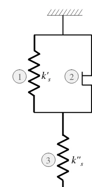
Three component models
A three component model can be composed of a combination of either two springs and a dashpot or two dashpots and a spring. A three component model as shown in Figure 2.8 is taken up, here, for further analysis. In this model a spring (spring constant = k′′)
is connected in series to a parallel arrangement of another spring (spring constant = k′) and a dashpot (viscosity =η
d). Identifying
k's ηd
k''s
1 2
3
Figure 2.8: A three-component model.
write,
σ =σ3 =σ1+σ2
ǫ1 =ǫ2
ǫ =ǫ3+ǫ2
k′
s =
σ1 ǫ1
ηd =
σ2
˙
ǫ2 ks′′ =
σ3 ǫ3
(2.18)
Combining all the above equations, one can obtain the constitutive relationship as,
σ+ ηd
k′
s+k′′s
˙
σ= k′sk′′s
k′
s+ks′′
ǫ+ k′′sηd
k′
s+ks′′
˙
time
Figure 2.9: Sinusoidal loading on rheological material in stress con-trolled mode.
The solution for the creep case (that is, ˙σ = 0) is obtained as,
ǫ=σo
The solution for the relaxation case (that is, ˙ǫ= 0) is obtained as,
σ =ǫok′′se
Under dynamic loading condition, a phase difference occurs be-tween the stress and the strain for rheologic materials. Figure 2.9 shows a schematic diagram of a stress controlled dynamic loading. The stress can be expressed as,
σ =σoeiωft (2.22)
where ωf is the angular velocity. The strain developed will have a
phase angle lag of δ. That is,
The energy dissipated per cycle per unit volume can be calculated
which is seen to be contributed from the out-of-phase portion. For elastic material δ= 0 indicating that the loss of energy due to dissipation will be zero. The complex modulus (E∗) can be written
as,
where, E′ is defined as the storage modulus, and E′′ as the loss
modulus. The dynamic modulus is defined as,
Ed=|E∗|=
p
(E′2+E′′2) (2.26)
The phase angle, δ can be obtained as,
δ =tan−1E′′
E′ (2.27)
The expression for Ed can be derived for any given model. For
example, incorporating σ = σoeiωft (that is, Equation 2.22) and ǫ=ǫoei(ωft−δ)(that is, Equation 2.23) in a three component model
(represented by Equation 2.19), and considering that ˙σ =iωfσand
Thus, the Ed (refer to Equation 2.26) is obtained as,
Ed=|E∗| (2.30)
=
(2ks+ksωf2η2)2 + (ωfηdks2)2
12
4k2
s +ωf2η2
(2.31)
and the phase angle (refer to Equation 2.27) is obtained as,
δ = tan−1 ωfηdks 2 +ω2
fη2d !
(2.32)
The Ed value of the asphalt mix is dependent on a number of
parameters, for example, aggregate gradation, asphalt binder vis-cosity, temperature, volumetric parameters, level of compaction, and so on. A number of predictive models have been developed to estimate the Edvalue of the asphalt mix from the known
parame-ters. Interested readers can refer to, for example, [19, 41, 149] etc. for more details.
Generalized models
In generalized models a large/infinite number of components are used. An example of a generalized Maxwell model is shown in Figure 2.10. Here, a number of Maxwell elements are connected in parallel. For this model, for the relaxation case, one can write,
ǫ1 =ǫ2 =· · ·=ǫi =· · ·=ǫo
σ=σ1+σ2+· · ·+σi+· · · (2.33)
Thus, the relaxation response can be written as,
σ(t) =X
∀i
σi =ǫo
X
∀i ksie
−kis
ηi d
ki s
2
1 3 4 i
Figure 2.10: A generalized Maxwell model.
ηdi
ksi
2 i
1
Figure 2.11: A generalized Kelvin model.
One can add various other components to the model, for example, if another spring is added in parallel, it is known as a Wiechert or Maxwell–Weichert model.
An example of a generalized Kelvin model is shown in Figure 2.111.
For this model, for a creep case, one can write,
σ1 =σ2 =· · ·=σi =· · ·=σo
ǫ =ǫ1+ǫ2+· · ·+ǫi+· · · (2.35)
1
Thus, the creep response can be written as,
ǫ(t) = X
∀i
ǫi =σo
X
∀i
1
ki s
1−e− kis ηidt
!
(2.36)
Other than the above examples of two-component, three-component and generalized models discussed, various other combi-nations of components are possible, and accordingly various mod-els have been proposed (for example, the Burger model, the Huet model, the Huet–Sayegh model and so on). Researchers use var-ious models to capture the time-dependent behavior of asphaltic material. One can refer to [55, 149] for example, for further study.
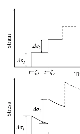
Linear viscoelasticity
A rheologic material can be called linearly viscoelastic, if the fol-lowing two conditions are satisfied.
• Homogeneity: For a stress controlled experiment, double the strain is observed at a particular time, if double the original stress has been applied. Similarly, for a strain controlled ex-periment, double the stress is observed at a particular time, if double the original strain has been applied.
• Superposition: The response at a given time to a number of individual excitations applied at different times is the sum of the responses that would have occurred by each excitation acting alone at those respective timings.
Time
t=ζ1
St
rai
n
ε1
ε2
t=ζ2
St
ress
Time
σ1
σ2
t=ζ1 t=ζ2
Figure 2.12: A strain-controlled thought experiment.
Figure 2.12 shows a strain controlled thought experiment on any rheologic material, like asphalt mix. In this experiment, an in-cremental strain of ∆ǫ1 is applied at time t = ζ1, then, another
incremental of strain ∆ǫ2 is applied at time t=ζ2 and so on.
If these cause increments of stress by ∆σ1, at time t = ζ1 and then, ∆σ2 att =ζ2 and so on, then, by using the above mentioned
conditions of linear viscoelasticity, one can add for all these time steps to obtain,
∆σ1 =Erel(t−ζ1) ∆ǫ1
∆σ2 =Erel(t−ζ2) ∆ǫ2
Assuming that the initial stress level of the material was zero (that
Thus, if a varying strain is applied to a rheologic material, it can be discretized into small time steps, and the above formulation (Equation 2.37) can be used to obtain the stress at a time t. In a similar manner, for a stress controlled experiment, one can derive,
ǫ(t) = ǫ|t=−∞+
X
∀i
Ccrp(t−ζi)∆σi (2.38)
For a continuous domain, these equations can be equivalently writ-ten as,
dζ dζ (for a strain controlled case)
(2.39)
dζ dζ (for a stress controlled case)
(2.40)
This is known as Boltzman’s superposition principle for linear viscoelastic material. By taking the Laplace transform to Equa-tions 2.39 and 2.40 one obtains [84],
σ(s) =sErel(s)ǫ(s) (2.41)
ǫ(s) = sCcrp(s)σ(s) (2.42)
where, σ(s), ǫ(s),Erel(s), Ccrp(s) are the stress, strain, relaxation
modulus and creep modulus in the Laplacian domain. From Equa-tions 2.41 and 2.42 one can write,
Ccrp(s)Erel(s) =
1
s2 (2.43)
It is interesting to note that in general Erel 6= Ccrp1 (except for
material maintains the above (given by, Equation 2.43) relation-ship in the Laplacian domain.
Equation 2.43 provides a link between the moduli value obtained from creep and relaxation tests for linear viscoelastic material. For a gluon expression for the creep response, it may be possi-ble to find out the expression for the relaxation response, with-out using the component structure of the model. Some illustra-tive problems are presented below. One may refer to, for example, [84, 161, 203] for further studies on the concepts of linear viscoelas-ticity and various inter-relationships that may exist among the parameters.
Example problem
A stress of magnitude σo is applied at t=ζ1 on a rheologic
mate-rial (which was initially stress-free) given as Equation 2.15, then withdrawn at t = ζ2 (refer to Figure 2.13). Predict the strain
re-sponse.
St
ress
Time
t = ζ1 t = ζ2 σo
Figure 2.13: A stress of magnitude σo applied at t = ζ1 on a
Solution
Equation 2.15 represents a Kelvin–Voigt model, whose creep re-sponse is given by Equation 2.16. From Equation 2.16 one can write,
Using Equation 2.38, one can write,
ǫ(t) = σo
The above strain response is shown schematically in Figure 2.14. Since the Kelvin–Voigt model has a spring and a dashpot con-nected in parallel (and no springs in series), the strain response does not show any (i) instantaneous deformation on the applica-tion of stress and (ii) instantaneous recovery on the withdrawal of stress (refer to Figure 2.14).
Example problem
A stress of magnitudeσois applied over a rheologic material (which
was initially stress-free) over a period ofζ1as shown in Figure 2.15. IfCcrp =
Time
S
tr
ai
n
ζ1 ζ2
No instantaneous deformation
No instantaneous recovery
Permanent deformation
Figure 2.14: Strain response of Kelvin–Voigt model with a stress of magnitude σo applied at t=ζ1 and then withdrawn at t =ζ2.
St
ress
Time
t = ζ1 σo
Figure 2.15: A stress of magnitude σo is applied linearly by t=ζ1
Solution
Creep compliance of a rheological model is given as
Ccrp(t) = t ηd
+ 1
ks
Find an expression for the relaxation modulus (Erel(t)).
Solution
After taking the Laplace transformation one obtains,
Ccrp(s) =
1
ηds2
+ 1
kss
Using Equation 2.43 one obtains,
Erel(s) =
By taking an inverse Laplace transform one obtains,
Erel(t) =kse
−ks
Example problem
A load of σ(t) = σoeiωft is applied on a three component model
(shown in Figure 2.8). The creep response of the model is given as Equation 2.20. Calculate the E∗ using Boltzman’s superposition
principle. Assume k′
s=ks′′=ks.
Solution
Considering Equation 2.20 and assuming k′
s =k′′s =ks
From Equation 2.40, one can write,
ǫ(t) =
It may be noted that the above expression for E∗ (that is,
Equa-tion 2.50) obtained using Boltzman’s superposiEqua-tion principle is the same as Equation 2.28.
Time–temperature superposition
Ccrp
ln (t)
T'' T'
T' > T''
t' t''
C'crp
C''crp
Figure 2.16: Schematic diagram illustrating the principle of time– temperature superposition.
compliance at different times and at two temperatures (say,T′ and
T′′, where,T′ > T′′) has been plotted schematically in Figure 2.16.
From Figure 2.16, it can be seen that at a given temperature, say at T′′, the C
crp at time t′ is lower than that of time t′′, (i.e., C′
crp < Ccrp′′ )—this is because, as time increases the strain keeps
on increasing. Further, it can be seen that at a given time, say at
t′, the C
crp at temperature T′′ is lower than that of temperature T′ (i.e.,C′
crp < Ccrp′′ )—this is because, if the temperature is higher,
the strain will be more at the same given time.
This behavior speaks for an equivalency that may exist between time and temperature, for example, the Ccrp measured at time t′′ at temperature T′′ is equal to the C
crp measured at time t′ at
temperature T′ (and its value is C′′
crp, as shown in Figure 2.16).
Thus, a relationship between the two time scales can be proposed
where, t′ can be called the reduced time of t′′ for shifting the test
temperature fromT′′ toT′, and α
T is called the time-temperature
shift factor. Obviously,αT is a function of these two temperatures,
so one of them can be treated as a standard temperature. Material for which αT value is not a dependent of time, can be called as a
thermorheologically simple material.
Certain formulations are proposed for calculation ofαT for
thermo-rheologically simple material. The following two formulae are typ-ically used for asphalt mixes. The Williams–Landel-Ferry (WLF) equation is given as [308],
loge(αT) =
−C1 T −Tref
C2+ T −Tref
(2.53)
where,loge(αT) is the natural logarithm ofαT,Tref is the reference
temperature, T is a temperature where αT is being determined,
and C1 and C2 are constants.
The Arrhenius Equation [85, 315] is given as,
loge(αT) =
where ∆His the apparent activation energy, andU is the universal gas constant.
If rheological tests are conducted at various temperatures2, it is
possible (and, more easily for a thermo-rheologically simple mate-rials) to develop the complete spectrum of rheologoical behavior of
2
the material at any specified reference temperature (Tref). This is
known as the master curve. Further, for dynamic testing it is pos-sible to establish equivalency with the frequency of loading (wf)
to time (for tests with static loading conditions) or temperature. One can, for example, refer to [149, 203, 219, 245, 291] on the (i) development of a master curve, (ii) interconversion between time, temperature, frequency, and (iii) techniques to obtain the curve fit parameters.
Discussions
Simple rheological models have been presented and some of these are used as descriptors of rheological behavior of asphalt mix [316, 321]. However, asphalt mix, as well as asphalt binder, show a more complex behavior in terms of their dependency on time, tempera-ture, and stress state. Further, asphalt mix is an anisotropic [292] and heterogeneous [10] material. Researchers have been trying to develop various models to capture the response and damage mech-anism of this complex material [17, 71, 76, 150, 157, 192, 242]. Interested readers may refer to [149, 156] for a review and further study on rheological modeling of asphalt mix (and asphalt binder).
2.3.2
Fatigue characterization
Bound materials (like asphalt mix) undergo fatigue damage due to repetitive application of load. In the laboratory, the loading may be applied in a stress or strain controlled manner on samples of various geometries. The repetitive loading may be flexural, axial, or torsional in nature; however, flexural fatigue loading is generally used for pavement engineering applications. Loading can be simple (where stress or strain amplitude level is maintained constant) or compound (where stress or strain amplitude level is varied during the course of testing) in nature.
Fat
ig
u
e
li
fe
Strain Stress ratio
En
d
u
ran
ce
l
im
it
Figure 2.17: Schematic diagram showing a possible fatigue behav-ior of bound materials in simple flexural fatigue testing.
generally expressed as the number of repetitions at which the elas-tic modulus reaches a predefined fraction of the original elaselas-tic modulus value [2, 176]. The stress ratio is defined as the ratio between the applied stress amplitude (for constant stress ampli-tude testing) and the flexural strength (known as the modulus of rupture) of the bound material. From Figure 2.17 it can be seen that if the strain (or stress ratio) level is high, the fatigue life is expected to be low and vice versa. Typically, strain is used as a parameter for fatigue characterization of asphalt material, and the stress ratio is used for cement concrete or cemented material. It has been observed that at a very low level of strain (or stress ra-tio), the sample does not fail due to such repetitive loading3 and
this is known as the endurance limit. This property later formed the basis of perpetual pavement design [209, 300].
3
For compound fatigue loading, the following empirical relationship generally satisfies,
X
∀i ni Ni
≈1 (2.55)
where,ni = the number of repetitions applied at a given strain (or
stress ratio) level, and Ni is the fatigue life of the material at that
strain (or stress ratio) level. Equation 2.55 was originally devel-oped based on experiments conducted on aluminum [200], and sub-sequently adopted in pavement engineering for characterizing the fatigue behavior of asphalt mix, cement concrete, and cemented material [67, 98, 124, 206, 217, 269, 281]. By using Equation 2.55 one assumes that fractional damages caused due to repetitions at various levels of strains (or stresses) are linearly accumulative [82].
A significantly large number of research studies is available on fatigue characterization of asphaltic material, covering the issues related to the mode/process of testing [2, 67, 191, 236, 269], fac-tors affecting the fatigue behavior [70, 176, 236], variability in test results [67, 236, 269], fracture and damage modeling of asphalt mix [57, 95, 150, 235], stiffness reduction [2, 176], asphalt heal-ing [118, 151], endurance limit [309] and so on. One can refer to articles, like [15, 156, 177] for an overview on the fatigue behavior of asphalt mix.
2.4
Cement concrete and cemented
material
An elastic modulus of cement concrete can be measured as a tan-gent modulus, a secant modulus or, dynamic modulus [207]. Fa-tigue performance of cement concrete is an important considera-tion in the concrete pavement design [1, 132, 206, 211, 217, 281, 285]. One can, for example, refer to textbooks such as [207, 208] etc. for a detailed study of the properties and characterization of cement concrete.
Cemented materials (generally locally available/marginal materi-als are utilized as the bound form) are bound material, hence these can be characterized in a manner similar to other bound material. Interested readers can refer to, for example [86, 106, 169, 217], for further study on the characterization of cemented material and its application in pavement construction.
2.5
Closure
Load stress in concrete
pavement
3.1
Introduction
Concrete pavements are often idealized as beams or plates on an elastic foundation. Numerous hypothetical springs placed at the bottom of the beam/plate represent the elastic foundation for such models. In this chapter, first the analysis of a beam resting on an elastic foundation is presented, followed by analysis of a thin plate resting on elastic foundation. Further, it is discussed how the plate theory can be utilized for analysis of an isolated concrete pavement slab (of finite dimension) resting on a base/sub-base.
3.2
Analysis of beam resting on elastic
foundation
A beam is a one-dimensional member. A schematic diagram of a beam (of unit width) resting on numerous springs with spring constant k (known as Winkler’s model, discussed later in
X
Z
Q
Figure 3.1: A beam resting on numerous springs is acted on by a concentrated load Q.
Section 3.2.1) subjected to a pointed loading Q at x = 0 is pre-sented as Figure 3.1. The free-body diagram of a portion of the beam (other than the load application point) is shown in Fig-ure 3.2. The moment (M) and shear force (V) are shown in the free-body diagram. The upward force of the spring on the element of length dx is ωkdx, where ω is the displacement of the beam in the Z direction. From Figure 3.2, using the force equilibrium one can write,
V −(V +dV) +kωdx= 0 (3.1)
Taking the moment equilibrium one obtains,
V = dM
dx (3.2)
Putting Equation 3.2 in Equation 3.1 and considering that
EIddx2ω2 = −M, (that is, for the Euler−Bernoulli beam) one
ob-tains,
EId
4ω
dx4 −kω= 0 (3.3)
X
M M+dM
V
V+dV
Z
dx
kwdx
Figure 3.2: Free-body diagram of dxelemental length of the beam presented in Figure 3.1.
applied to foundation engineering [109, 136, 144, 247]. The general solution of Equation 3.3 is given as,
ω =eλx(c1cosλx+c2sinλx)+e−λx(c3cosλx+c4sinλx) (3.4)
where,λ = k 4EI
14
, and c1, c2,c3 and c4 are constants. These con-stants can be determined from the boundary conditions pertaining to the specific geometry of the problem. Considering one side of the beam (for instance, the right side) with respect to the load application point of the infinite beam (as shown in Figure 3.1), one can write the following boundary conditions and subsequently derive the following results [109].
• limx→∞ω = 0. This condition leads to c1 = c2 = 0. Thus,
the equation reduces to ω =e−λx(c3cosλx+c4sinλx)
• Due to symmetry, dωdx |x→0= 0 . This leads to c3 = c4 = c
(say)
to the downward force Q applied, that is, 2R∞
0 kω dx = Q.
This leads to c= Qλ2k
Hence, the expression for deflection of an infinite beam resting on an elastic foundation is obtained as,
ω = Qλ
2ke
−λx(cosλx+ sinλx) (3.5)
It may be noted that the developed equation (Equation 3.5) is valid only for the right side (i.e., x ≥ 0) of the infinite beam. In a similar manner, an expression can be developed for the left side of the beam. Then, the first boundary condition changes as, limx→−∞ = 0; the other two conditions remain the same. From
these boundary conditions, the constants are obtained as c3 =
c4 = 0, and c1 =−c2 = Qλ2k. The equation (for the left side of the infinite beam from x= 0) takes the form of,
ω = Qλ
2ke
λx(cosλx−sinλx) (3.6)
Equations 3.5 or 3.6 can be utilized (by successive differentiation) to obtain the rotation, bending moment, and shear profile [109]. The maximum deflection is under the load and is obtained as,
ωmax = Qλ
2k (3.7)
In case there is a uniformly distributed loading (instead of point loading) of q per unit length, the deflection can be obtained by integration.
For the loading diagram shown as in Figure 3.3, the deflection at
AA′ (ω
AA′) can be obtained by using superposition of deflection
n m
A'
dx x
A
q
Z
X
Figure 3.3: Analysis of an infinite beam with distributed loading.
If the section AA′ is outside the loaded area (of length n +m),
Equation 3.5 or 3.6 needs be used with appropriate integration limits. Further, the beam can be assumed as semi-infinite (that is, the beam has a definite ending at one side, and the other side is infinite), or finite (that, is the beam has a finite length). In such cases, an appropriate boundary condition can be used. Alterna-tively, one can solve it as a superposition of two infinite beams. One can refer to [109, 247], for example, for the details of the various approaches.
Such one dimensional analysis is useful, for example, for analysis of the problem of the dowel bar. Figure 3.4 illustrates how a single dowel bar can be idealized as a finite beam resting on an elastic foundation. However, additional considerations are involved in the dowel bar analysis problem (refer to Figure 3.4), for example, (i) there is a discontinuity of support in the middle portion, (ii) one side of the dowel bar is embedded in concrete but the other side is free to move horizontally, (iii) the wheel load does not directly act on the dowel bar, etc. Interested readers can refer to past works by Friberg [87, 88] and Bradbury [27] and a relatively recent study by Porter [223] on dowel bar analysis and the assumptions involved.
Wheel
Concrete slab Concrete slab Dowel bar
(a) Schematic diagram of a dowel bar in a concrete slab
(b) Idealized representation of dowel bar Q
Gap= zs
Figure 3.4: Idealization of a dowel bar for analysis.
(of q per unit length, which may include self-weight) and arbi-trary foundation support (of pper unit length) condition (refer to Figure 3.5) can be written as:
dV
dx =p−q (3.9)
Or,
EId
4ω
dx4 =q−p=q
∗ (3.10)
q
p
where, q∗ is the net loading per unit length in the downward
di-rection. Depending on the foundation support, the expression for
p may become different. It may be noted that ifp= 0, it becomes equivalent to the beam bending equation, without any spring sup-port. Winkler, Pasternak, and Kerr are the examples of different types of supports, and are briefly discussed in the following.
3.2.1
Beam resting on a Winkler foundation
Unconnected (linear) springs are known as Winkler’s springs [124, 142, 144, 182]. Formulation for a beam resting on a Winkler spring for a pointed loading was already discussed in the beginning of this section (Section 3.2). That is, for a Winkler spring, p = kω. Thus, a beam resting on a Winkler spring subjected to loading q
(following Equation 3.3) can be represented as,
EId
4ω
dx4 =q−kω (3.11)
The Winkler spring constant (k) used here in the formulation in-dicates the pressure needed on the spring system to cause unit displacement.1 Its unit is therefore MPa/mm. As discussed in
Sec-tion 2.2, the modulus of subgrade reacSec-tion (k) is also the pressure needed to cause unit deformation to the medium (that is, subgrade or sub-base or base layer). Thus, the spring constant used in the present formulation is conceptually equivalent to the modulus of subgrade reaction of the supporting layer.
One can refer to the paper written by Terzaghi [270] for a de-tailed discussion on the evaluation of thek value. Non-uniqueness of the modulus of the subgrade reaction in terms of the prediction of the (i) deflected shape (especially at the edges and corners of the slab) or (ii) stresses, is an issue raised by past researchers.
1
X
Z
(b) Free body diagram of an element of the shear layer V'+dV' pdx
V'
kwdx
dx
Shear layer
(a) A beam resting on a Pasternak foundation
Figure 3.6: A beam resting on a Pasternak foundation and a free-body-diagram of the shear layer.
One can, for example, refer to [62, 117, 233] for discussions on the issues involved. This has prompted researchers in the past to develop multi-parameter models to capture the response of struc-tures resting on soil. Some of these are discussed in the following.
Beam resting on a Pasternak foundation
In a Pasternak foundation, it is assumed that there is a hypothet-ical shear layer placed at the top of the spring system (refer to Figure 3.6(a)). Thus, considering the equilibrium of an element of length dx of shear layer (refer to Figure 3.6(b)), one can write,
pdx−V′ + (V′+dV′)−kωdx= 0
p=kω− dV
′