Multiplicative Updates for Learning with
Stochastic Matrices
Zhanxing Zhu, Zhirong Yang⋆, and Erkki Oja
Department of Information and Computer Science, Aalto University⋆⋆
P.O.Box 15400, FI-00076, Aalto, Finland
{zhanxing.zhu}@gmail.com,{zhirong.yang,erkki.oja}@aalto.fi
Abstract. Stochastic matrices are arrays whose elements are discrete probabilities. They are widely used in techniques such as Markov Chains, probabilistic latent semantic analysis, etc. In such learning problems, the learned matrices, being stochastic matrices, are non-negative and all or part of the elements sum up to one. Conventional multiplicative updates which have been widely used for nonnegative learning cannot accommo-date the stochasticity constraint. Simply normalizing the nonnegative matrix in learning at each step may have an adverse effect on the con-vergence of the optimization algorithm. Here we discuss and compare two alternative ways in developing multiplicative update rules for stochastic matrices. One reparameterizes the matrices before applying the multi-plicative update principle, and the other employs relaxation with La-grangian multipliers such that the updates jointly optimize the objective and steer the estimate towards the constraint manifold. We compare the new methods against the conventional normalization approach on two applications, parameter estimation of Hidden Markov Chain Model and Information-Theoretic Clustering. Empirical studies on both synthetic and real-world datasets demonstrate that the algorithms using the new methods perform more stably and efficiently than the conventional ones.
Keywords: nonnegative learning, stochastic matrix, multiplicative up-date
1
Introduction
Nonnegativity has shown to be a useful constraint in many machine learning problems, such as Nonnegative Matrix Factorization (NMF) (e.g. [1–3]) and clus-tering (e.g. [4, 5]). Multiplicative updates are widely used in nonnegative learning problems because they are easy to implement, while naturally maintaining the nonnegativity of the elements to be learned after each update. Consider a matrix problem: suppose we are minimizing an objective functionJ(W) over a nonneg-ative matrix W, that is, Wik ≥ 0 for all (i, k). Multiplicative update is easily
⋆corresponding author
⋆⋆ This work is supported by the Academy of Finland (grant numbers 251170 and
derived from the gradient∇=∂J/∂W. The conventional multiplicative update rule is given by
Wik←Wik
∇−
ik
∇+ik, (1)
where∇+ and∇− are the positive and (unsigned) negative parts of∇,
respec-tively, i.e.∇=∇+− ∇−.
When dealing with probabilistic problems such as Markov Chains, the matrix elements are discrete probabilities. Then, in addition to the nonnegativity con-straint, some or all entries of such matrices must sum up to one. Such matrices are called stochastic matrices. Given a nonnegative matrix W, there are three typical stochasticities in nonnegative learning:
– (left stochastic) or column-sum-to-one:PiWik= 1, for allk,
– (right stochastic) or row-sum-to-one:PkWik= 1, for alli,
– (vectorized stochastic) or matrix-sum-to-one: PikWik= 1.
The multiplicative update rule in Eq. (1) cannot handle as such the stochas-ticity constraints. A normalization step is usually needed to enforce the unitary sum (e.g. [6–8]). However, this simple remedy may not work well with the mul-tiplicative updates and may cause unstable or slow convergence. There is little literature on adapting the multiplicative update rules for stochastic matrices.
We focus here on how to develop multiplicative update rules for stochastic matrices in nonnegative learning in a general way. For clarity we only solve the right stochastic case in this paper, while the development procedure and discussion can easily be extended to the other two cases.
We present two approaches in Section 2. The first applies the principle of multiplicative update rules in a reparameterized space, while the second per-forms multiplicative updates with the relaxed constraints by using Lagrangian multipliers. While both approaches are quite generic and widely used, they have not been applied in detail on stochastic matrix learning problems. In Section 3, these methods demonstrate their advantages in terms of stability and conver-gence speed over the conventional normalization approach in two applications, estimating Hidden Markov Chain Models and clustering, on both synthetic and real-world data. Section 4 concludes the paper.
2
Multiplicative updates for stochastic matrices
2.1 Normalization
The simplest approach for maintaining the constraints is re-normalization, which has conventionally been used for updating stochastic matrices (e.g. [6, 7]). After each multiplicative update by Eq. (1), this method normalizes the matrix:Wik←
Wik/PbWib. However, as shown in Section 3.2, the normalization method often
2.2 Reparameterization
Alternatively, we reparameterize the right stochastic matrix W into a non-stochastic matrix U via Wsb = Usb/PaUsa. We can then optimize over U
without the stochasticity constraints, instead ofW. For notation brevity, in this paper, we denote∇+and∇−as positive and (unsigned) negative gradient parts
of the objective function J(W) forW. For the gradients of other matrices, we use subscripts to differentiate those ofW, for example,∇+
U and∇−U.
With the reparameterization, we have ∂Wsb
∂Ust = is the Kronecker delta function. Applying the chain rule, the derivative of J with respect toU is
∂J
This suggests multiplicative update rules forU andW:
Ust←Ust
The Lagrangian technique, as a well-known method to tackle constraints in opti-mization, can be employed here to relax the stochasticity constraints. Given the set of equality constraints PkWik−1 = 0, i = 1, . . . , m for a right stochastic
matrix, the relaxed objective function can be formulated by introducing La-grangian multipliers{λi}mi=1:Je(W,{λi}mi=1) =J(W)−
. Inserting the preliminary update rule into
the constraint PbWib′ = 1, we have
.Putting them back to the preliminary rule,
we haveWik′ =Wik
There is a negative term−Bik in the numerator, which may cause negative
en-tries in the updated W. To overcome this, we apply the “moving term” trick [9–12] to resettleBik to the denominator, giving the final update rule
Wik←Wik
∇−
ikAik+ 1
∇+ikAik+Bik
. (4)
The final update rule reveals that there are two forces, weighted byAik, in
the update procedure of W. One keeps the original multiplicative update rule Wik ←Wik∇−ik/∇
+
ik, and the other steers the matrix to approach the manifold
specified by the stochasticity constraints. Incorporating the two forces into one update rule can ultimately optimize the matrix W and fulfill the constraints approximately as well.
Moreover, if there exists a certain auxiliary upper-bounding function (see e.g. [1, 9]) forJ(W) and minimization of the auxiliary function guarantees that J(W) monotonically decreases under multiplicative updates, we can easily de-sign an augmented auxiliary function for Je(W,{λi}) by the principle in [9] to
keep the relaxed objective function descending under the update rule (4). This can theoretically ensure the objective function convergence of multiplicative up-date rules for stochastic matrices.
3
Applications
3.1 Parameter estimation in HMM
AHidden Markov Model (HMM) chain is widely used for dealing with temporal or spatial structures in a random process. In the basic chain model, s(i) de-notes the hidden state at time i, taking values from S ={1,2, . . . , r}, and its corresponding observed output is denoted byx(i). The state joint probability is S(s1, s2) =P(s(i) =s1, s(i+ 1) =s2). The factorization of the joint probability of two consecutive observations Xb(x1, x2) = P(x(i+ 1) = x2, x(i) =x1), can be expressed as Xb(x1, x2) = Ps1,s2P(x1|s1)S(s1, s2)P(x2|s2). For the discrete and finite random variable alphabet |X | = m, Xb forms an m×m vectorized stochastic matrix. Then, the above factorization can be expressed in matrix form: Xb =P SPT,whereXb ∈Rm×m
+ , P ∈Rm+×r andS∈Rr+×r.
The matrixXb is generally unknown in practice. Based on the observations, x(1), . . . , x(N),Xb is usually approximated by the joint normalized histogram
X(x1, x2) = 1 N−1
nX−1
i=1
δ(x(i) =xi)δ(x(i+ 1) =x2), (5)
whereδis Dirac delta function. With the Euclidean distance metric, the NMF op-timization problem can be formulated as minP≥0,S≥0J(P, S) = 12kX−P SPTk2, subject toPiPis= 1,PstSst= 1 fors= 1, . . . , r.
Lakshminarayanan and Raich recently proposed an iterative algorithm called NNMF-HMM for the above optimization problem [13]. Their method applies normalization after each update of P and S, which is in turn based on matrix pseudo-inversion and truncation of negative entries.
Here we solve the HMM problem by multiplicative updates. First, we de-compose the gradients ofJ to positive and negative parts:∇P =∇+P− ∇
−
P and
∇S=∇+S− ∇
−
S where∇
+
P =P SPTP ST+P STPTP S,∇
−
P =XP ST+XTP S,
∇+S =PTP SPTP, and ∇−
Table 1. Comparison of convergence time (in seconds) and final objective on (top) synthetic dataset and (bottom) English words dataset. Results are in the form mean
±standard deviation.
Methods NNMF-HMM norm.-HMM repa.-HMM rela.-HMM Time 3.52±2.10 1.00±0.44 1.84±1.04 1.89±0.56 Objective 4×10⁻³
±1×10⁻⁹
7×10⁻⁶
±9×10⁻⁹
4×10⁻⁵
±9×10⁻⁵
7×10⁻⁶
±9×10⁻⁹
Methods NNMF-HMM norm.-HMM repa.-HMM rela.-HMM Time 0.15±0.09 2.94±1.43 2.53±1.28 2.89±0.62 Objective 6×10⁻³
±2×10⁻³
8×10⁻⁴
±0.2×10⁻⁴
9×10⁻⁴
±1×10⁻⁴
8×10⁻⁴
±0.2×10⁻⁴
are then formed by inserting these quantities to the rules in Section 2. Note that P is left stochastic andSis vectorized stochastic. Some supporting formulae for these two cases are given in the appendix.
We have compared the multiplicative algorithms against the implementation in [13] on both synthetic and real-world data. First, a data set was generated under the same settings as in [13]. That is, we constructed an HMM withr= 3
states and a transition matrix X(s2|s1) =
0 00 0.9 01.1 1 0 0
. Next, x′
was sampled
based on the conditional distributions x′|s= 1∼ N(11,2), x′|s= 2∼ N(16,3) and x′|s = 3 ∼ Uniform(16,26). Then x was generated by rounding x′ to its nearest integer. We sampled N = 105 observations and calculated the joint probability normalized histogram matrixX by Eq. (5).
The iterative algorithms stop when kP−PoldkF
kPkF < ǫand
kS−SoldkF
kSkF < ǫ, where k · kF stands for Frobenius norm and ǫ = 10−6. We run the algorithms 50
times with different random initialization forP andS. All the experiments are performed on a PC with 2.83GHz CPU and 4GB RAM. Results are given in Table 1 (top), from which we can see that the three methods with multiplicative updates are faster and give better objectives than NNMF-HMM.
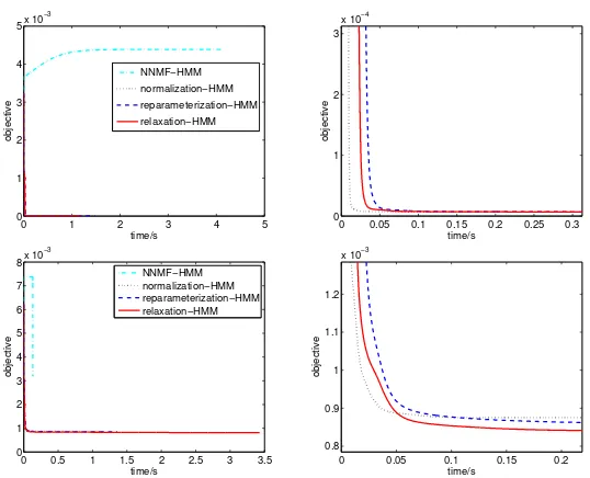
For one group of random implementations, we compare their convergence speeds, i.e, objective value as a function of time, in Fig. 1 (top). We can ob-serve that NNMF-HMM algorithm gets stuck into a high objective. The other three algorithms converge much faster and have similar convergence speed while satisfying the stochasticity constraints.
0 1 2 3 4 5 0
1 2 3 4 5x 10
−3
time/s
objective
NNMF−HMM normalization−HMM reparameterization−HMM relaxation−HMM
0 0.05 0.1 0.15 0.2 0.25 0.3 0
1 2 3
x 10−4
time/s
objective
0 0.5 1 1.5 2 2.5 3 3.5 0
1 2 3 4 5 6 7 8x 10
−3
time/s
objective
NNMF−HMM normalization−HMM reparameterization−HMM relaxation−HMM
0 0.05 0.1 0.15 0.2 0.8
0.9 1 1.1 1.2
x 10−3
time/s
objective
Fig. 1.Objective evolution of the compared algorithms in HMM parameter estimation on (top) synthetic data set and (bottom) English words. The right sub-figures are the zoom-in plot for early epochs.
3.2 Nonparametric Information Theoretic Clustering
Next, we demonstrate another application of the proposed methods to a nonneg-ative learning problem beyond matrix factorization:Nonparametric Information Clustering (NIC) [4]. This recent clustering approach is based on maximizing the mutual information between data points and formulates a clustering crite-rion analogous tok-means, but with locality information enhanced.
Given a set of data points{x1, x2, . . . , xN} and the number of clusters nC,
denote the cluster ofxi byC(xi) =ci, and the number of points assigned to the
kth cluster bynk. NIC minimizes the following score as the clustering criterion:
JN IC(C) =Pknk1−1Pi6=j|ci=cj=klogkxi−xjk2. Faivishevsky and Goldberger
[4] proposed a greedy algorithm to optimize the score function JN IC(C).
Ini-tialized by a random partition, the greedy algorithm repeatedly picks a data point and determines its cluster assignment that maximizes the score function JN IC(C). Note that for each data point, the greedy algorithm has to recompute
the score function, which is expensive for large data sets.
To overcome this issue, we reformulate the hard clustering problem into a soft version such that differential calculus in place of combinatorial optimization can be used. Moreover, we use batch updates of cluster assignments for all data points. First, we relax the score function JS
N IC =
P
kp(k)
P
ijp(i|k)p(j|k)Dij
abbrevi-−1 −0.5 0 0.5 1
greedy sequential algorithm of NIC
−1 −0.5 0 0.5 1
Fig. 2. Clustering analysis for a synthetic dataset (top left) using five algorithms: greedy algorithm (top middle), normalization (top right), reparameterization (bottom
left), relaxation (bottom middle) andk-means (bottom right).
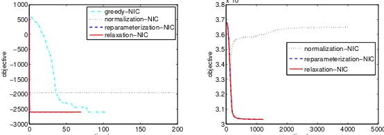
0 50 100 150 200
0 1000 2000 3000 4000 5000 3
Fig. 3.Objective evolution of a typical trial of compared NIC algorithms: (left) syn-thetic dataset and (right) pen digit dataset.
ates the dissimilarity matrix for the whole data set, withDij = logkxi−xjk2.
In clustering, our aim is to optimize conditional probability p(k|i), the soft as-signment tokth cluster for data pointxi. Applying the Bayes theorem, we have
p(i|k) = Pp(k|i)p(i)
For notational simplicity, we define the assignment matrixWik=p(k|i). The
NIC model can thus be reformulated as the following nonnegative optimization problem: minW≥0JN ICS (W) = N1 construct multiplicative updates forW as described in Section 2. The iterative algorithms terminate when kW−WoldkF
kWkF <10
−5.
Table 2.Comparison of convergence time and final objective on synthetic clusters.
Methods greedy norm.-NIC repa.-NIC rela.-NIC k-means Time (s) 80.83±17.75 535.11±37.25 7.22±7.06 6.98±6.94 0.03±0.05 Objective−2.60×10³
±0−2.53×10³
±204−2.60×10³
±0.01−2.60×10³
±0.01−1.79×10³
±490 Purity 0.99±0 0.97±0.06 0.99±0 0.99±0 0.72±0.14
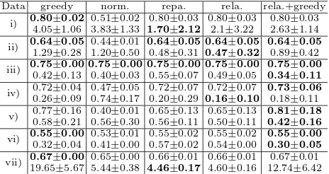
Table 3.Clustering performance for the five compared methods on datasets i) ecoli, ii) glass, iii) parkinsons, iv) iris, v) wine, vi) sonar, and vii) pima. Each cell shows
the mean and standard deviation of clustering purity (the first line) and converged
time (the second line, in seconds). The abbreviationsnorm.,repa., andrela.stand for normalization, reparameterization, and relaxation, respectively. Bold numbers indicate the best in each row.
Data greedy norm. repa. rela. rela.+greedy
i) 0.80±0.02 0.51±0.02 0.80±0.03 0.80±0.03 0.80±0.03 4.05±1.06 3.83±1.33 1.70±2.12 2.1±3.22 2.63±1.14 ii) 0.64±0.05 0.44±0.01 0.64±0.05 0.64±0.05 0.64±0.05
1.29±0.28 1.20±0.50 0.48±0.31 0.47±0.32 0.89±0.42 iii) 0.75±0.00 0.75±0.00 0.75±0.00 0.75±0.00 0.75±0.00
0.42±0.13 0.40±0.03 0.55±0.07 0.49±0.05 0.34±0.11 iv) 0.72±0.04 0.47±0.05 0.72±0.07 0.72±0.07 0.73±0.06 0.26±0.09 0.74±0.17 0.20±0.29 0.16±0.10 0.18±0.11 v) 0.77±0.16 0.40±0.01 0.65±0.13 0.65±0.13 0.81±0.18
0.58±0.21 0.56±0.30 0.56±0.11 0.50±0.11 0.42±0.16 vi) 0.55±0.00 0.53±0.01 0.55±0.02 0.55±0.02 0.55±0.00 0.32±0.04 0.41±0.00 0.57±0.02 0.54±0.00 0.30±0.05 vii) 0.67±0.00 0.65±0.00 0.66±0.01 0.66±0.01 0.67±0.01
19.65±5.67 5.44±0.38 4.46±0.17 4.60±0.16 12.74±6.42
cluster has 300 data points. A typical run of the compared NIC algorithms is shown in Fig. 3 (left). We can see that the normalization method gets stuck and returns a high objective. The other three methods can find better NIC scores, whereas the greedy algorithm requires much more time to converge. By contrast, reparameterization and relaxation achieve nearly the same efficiency. We have repeated the compared algorithms 50 times with different random initializations. The means and standard deviations of the running time and objective are shown in Table 2, which again shows the efficiency advantage of the algorithms using the proposed methods.
We validate the converged estimates by checking their corresponding clus-tering results. From Fig. 2,k-means and normalization methods split the large circle into several parts and fail to identify the four pies in the middle. The NIC algorithms can correctly identify the five clusters. The clustering performance is quantified by thepuritymeasurement, which is calculated byN1 Pkmax1≤l≤qnlk,
withnl
k the number of samples inkth cluster that belong to true classl. A larger
purity usually corresponds to better clustering performance. The last row in Ta-ble 2 indicates that the new algorithms are not only fast but are aTa-ble to produce satisfactory clustering results.
We have also tested the compared algorithms for NIC on several real-world datasets selected from the UCI Machine Learning Repository1. The results are shown in Table 3. We can see that in six out of seven datasets, the reparameteri-zation and relaxation methods can achieve similar purity as the greedy algorithm
Table 4. Comparison of convergence time, final objective and purity on pen digits dataset.
Methods greedy norm.-NIC repa.-NIC rela.-NIC k-means Time (s) − 4509±328 1276±41 1274±38 0.7±0.4 Objective − 36445±51 30457±177 30457±177 30812±285
Purity − 0.37±0.001 0.73±0.04 0.73±0.04 0.68±0.04
but with less learning time. For the wine dataset, though the purities obtained by the proposed methods are inferior to those by the greedy algorithm, we can use the relaxation (or reparameterization) method as initialization, followed by the greedy approach. This way we can achieve satisfactory purity but still with reduced learning time. Surprisingly, this hybrid method produces even better clustering purities for the datasetsirisandwine. By contrast, the normalization method is again unstable and its clustering purity is much lower than the others for four out of seven datasets.
The efficiency advantage brought by the proposed method is clearer for larger datasets, e.g.pima. Furthermore, we applied the compared methods to an even larger real world data set, “Pen-Based Recognition of Handwritten Digits Data Set” also from the UCI Repository. This data set contains 10992 samples, each of which is 16-dimensional. In clustering the digits, the two proposed methods can achieve purity 0.73 except the normalization approach (purity 0.37), see Table 4. However, the greedy algorithm needs more than one day to converge, while the proposed reparameterization and relaxation multiplicative updates can converge within 20 minutes, as compared with the normalization method in the right panel of Fig. 3.
4
Conclusions
We have introduced two methods, reparameterization and relaxation, for mul-tiplicatively updating stochastic matrices. Both methods share the property of good convergence speed and can fulfill the stochasticity constraints. They out-perform the conventional normalization method in terms of stability. We have applied the proposed algorithms to two applications, parameter estimation in HMM and NIC clustering. Experimental results indicate that the proposed two methods are advantageous for developing multiplicative algorithms for nonneg-ative learning with stochastic matrices.
In future work, we would like to investigate the theoretical proof on the con-vergence of reparameterization and relaxation methods, which can be handled by constructing proper auxiliary functions. Moreover, the connection between the proposed methods and the Dirichlet process prior deserves further investigation.
A
Formulae for left and vectorized stochastic matrices
In reparameterization method, for left stochastic matrix,
∂J ∂Ust
= ∇
+
st
P
aUat
+(U
T∇−)
tt
(PaUat)2
− ∇
−
st
P
aUat
+(U
T∇+)
tt
(PaUat)2
for vectorized stochastic matrix,
In relaxation method, for left stochastic matrix,
Aik=
and for vectorized stochastic matrix,
Aik=
1. Dhillon, I.S., Sra, S.: Generalized nonnegative matrix approximations with breg-man divergences. In: Advances in Neural Information Processing Systems. Vol-ume 18. (2006) 283–290
2. Choi, S.: Algorithms for orthogonal nonnegative matrix factorization. In: Proceed-ings of IEEE International Joint Conference on Neural Networks. (2008) 1828–1832 3. Cichocki, A., Zdunek, R., Phan, A.H., Amari, S.: Nonnegative Matrix and Tensor Factorizations: Applications to Exploratory Multi-way Data Analysis. John Wiley (2009)
4. Faivishevsky, B., Goldberger, J.: A nonparametric information theoretic clustering algorithm. In: The 27th International Conference on Machine Learning. (2010) 5. Jin, R., Ding, C., Kang, F.: A probabilistic approach for optimizing spectral
clus-tering. In: Advances in Neural Information Processing Systems. (2005) 571–578 6. Lee, D.D., Seung, H.S.: Learning the parts of objects by non-negative matrix
factorization. Nature401(1999) 788–791
7. Ding, C., Li, T., Peng, W.: On the equivalence between non-negative matrix factorization and probabilistic latent semantic indexing. Computational Statistics
and Data Analysis52(8) (2008) 3913–3927
8. Mørup, M., Hansen, L.: Archetypal analysis for machine learning. In: IEEE In-ternational Workshop on Machine Learning for Signal Processing (MLSP), IEEE (2010) 172–177
9. Yang, Z., Oja, E.: Linear and nonlinear projective nonnegative matrix factorization.
IEEE Transaction on Neural Networks21(5) (2010) 734–749
10. Yang, Z., Oja, E.: Unified development of multiplicative algorithms for linear and quadratic nonnegative matrix factorization. IEEE Transactions on Neural
Networks22(12) (2011) 1878–1891
11. Yang, Z., Oja, E.: Quadratic nonnegative matrix factorization. Pattern Recognition
45(4) (2012) 1500–1510
12. Yang, Z., Oja, E.: Clustering by low-rank doubly stochastic matrix decomposition. In: International Conference on Machine Learning (ICML). (2012)