Growing Urban Roads
DANIEL YAMINS
Faculty of Arts and Sciences, Harvard University, Cambridge, MA 02138, USA; Los Alamos National Laboratory, Earth and Environmental Sciences (EES-6) and Center for Nonlinear Studies, Los Alamos, NM 87545, USA email: [email protected]
STEEN RASMUSSEN
Los Alamos National Laboratory, Earth and Environmental Sciences (EES-6) and Center for Nonlinear Studies, Los Alamos, NM 87545, USA; Santa Fe Institute, 1399 Hyde Park Road, Santa Fe, NM 87501, USA
email: [email protected]; [email protected]; www.lanl.gov/home/steen
DAVID FOGEL
Department of Geography, University of California Santa Barbara, Santa Barbara, CA 93106, USA email: [email protected]
Abstract
We present a simple simulation of road growing dynamics that can generate global features as belt-ways and star patterns observed in urban transportation infrastructure. The road growing dynamics consist of two steps: Identifying the maximum transportation potential bewteen two locations within the city, followed by the generation of the least expensive road between these two locations. The simulation defines a previously missing component for modeling the co-evolution of urban settlement- and road systems as it can directly be coupled to existing urban settlement simulations.
Keywords: transportation network evolution, corridor location, urban dynamics, network growth algorithm
1. Introduction
Any major city consists of an urban system of systems including buildings (settlement), transportation network, energy generation and distribution networks, communication net-works, waste-, food-, and water distribution systems, surface and subsurface water flow, the local atmosphere, the geological setting, internal and surrounding ecosystems, economic zones, demographics, and many others as discussed under the Los Alamos Urban Security Initiative (Heiken et al., 2000; http://www.ees.lanl.gov/EES5/Urban Security/). Perhaps the two most important human-made subsystems determining urban form and structure are the settlements and the transportation infrastructure. In this work we focus on the long term dynamics and structure of the latter.
Lombard and Church, 1993; Goodchild, 1997). Urban settlement dynamics have been dis-cussed in a formal setting for many years by many groups ranging from purely theoretical to applied planning tools, including diffusion-limited aggregation, correlated perculation, cellular automata, agent based, and dynamic GIS models (Benenson and Portugali, 1997; Benguigui, 1995; Benguigui and Daoud, 1995; Candau et al., 2000; Clarke et al., 1997; Clarke and Gaydos, 1998; Couclelis, 1996; Makse et al., 1995, 1998; Sanders et al., 1997; Takeyama, 1996; Wu, 1998; Xie, 1996). The road building dynamics to be presented here can be coupled to any of these settlement simulations that explicitly take into account the transportantion infrastructure. Also the dynamics of existing urban transportation in-frastructure has attracted much attention e.g. through the large scale TRANSIMS project (http://transims.tsasa.lanl.gov; Nagel et al., 1997) as well as many of the contributions in this special volume.
In this work we present a simple two step method for simulating the growth of urban trans-portation networks. The first step is the selection of appropriate locations to be connected by transport links based on a potential function. The second step is the road building process itself, which is a cost-based algorithm. This second step has been discussed in great detail previously in Church et al. (1992), Lombard and Church (1993), and Goodchild (1977), but in a different context as the “corridor location problem.” In the corridor location prob-lem various cost-based algorithms are defined for locating the optimal connection pathway between two points in a geographical landscape. The algorithms developed by Lombard, Church and Goodchild have been used in various situations within geographical modeling, such as Ehlschlaeger and Shortridge (1996) and Miller (1999). In our work, we use a min-imalistic road growing algorithm that relates to the potential function used in the first step, the pair-location algorithm, to obtain qualitiative information about the global nature of road growing dynamics in urban areas. The more complex corridor location algorithms are not necessary to generate the global features observed in urban road networks. This simple method should especially be adaptable to studying the global qualitative properties of the long term co-evolution of the transport network with the larger settlement system that the road system serves.
Yet another perspective is taken in Schweitzer et al. (1998) where a fixed set of origin and destination points (e.g. within a city or between cities) are assumed whereafter an opti-mal transportantion infrastructure between these points is generated using an evolutionary method. Finally it should be noted that trails and possibly also urban roads could also be generated using “active walker” methods (Schweitzer, 1997) inspired from ant foraging behavior.
2. The representation
2.1. Overview
whereSt represents the system state at timet and the first arrowi represents a (random)
seeding process which contains land use, land cover and road information. The second arrow (l) represents the generation of new land use (settlements) for instance as discussed in White et al. (1997), Clarke et al. (1997), and Andersson et al. (2002). No new roads are build in this process although existing roads do interact with the land use dynamics and thus partially determine the land use evolution. The next arrow (g) represents the road evolution—the growing of new roads. The settlement pattern is assumed to be constant in this process and is the main factor determining the location of new roads. In fact, this road growing process is itself of an iterative nature as will be clear later. Next co-evolution iteration starts asloperates onSt+1followed bygoperating onSt′+1etc.
To make our analysis as simple as possible we only discuss and report the properties of the road growing dynamics, denotedgin Eq. (1). For simplicity as an initial condition we also assume an existing, homogeneous urbanized area and only generate the main transportation infrastructure within this urbanized area—or through a simple, externally driven urbanization to be introduced later. Obviously, this is not a realistic assumption, but it makes the problem tractable and a later integration with an existing settlement dynamics simulation as discussed in Eq. (1) is straight forward. Perhaps this way of growing roads within an existing city is most appropriately compared with a transportation retro-fitting situation as for example the addition of express- and free ways in many larger cities in the 1950’s.
The basic idea behind the road growing dynamics in our system is simple and only assumes:
(i) A local transport by diffusion and
(ii) A non-local transport by connected transportation links (roads) which grow between urban areas with high transportation potential. The static structure of the model is a 2-D lattice (which will be discussed in 2.2 below).
This view on road transport is analogous to what is observed in many physical and biological systems including river systems and tissues. The urban transport demand is driven by a transportation potential which is defined as the total non-connected “urban mass.” Loosely speaking is the part of the urban area which cannot be accessed by existing roads. The road growing dynamics is constrained by two obvious costs: (a) The cost of having roads pass through existing urbanized areas, the denser an area, the more costly, (b) and the cost of having roads wiggle around dense areas; the longer the road, the more costly it is to construct and the longer transportation time will result, thus decreasing the vale of the link. In the following we shall make all of the above more precise.
2.2. The lattice
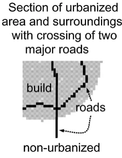
In this section, we will describe the static structure used in the model. Let us assume that we can represent the urban setting with its settlements and transportation infrastructure as different states on a 2-D latticeL(figure 1). Letxi denote the first coordinate andxj the
Figure 1. Illustration of the representation of two major intersecting urban roads on the 2-D latticeL. Black indicates transportation infrastructure, light grey indicates urbanized areas and white indicates non-urbanized (non-build) areas. See text for details.
urbanized land and 2 indicates major transportation infrastructure. A road is a connected set of nodes (=transportation links) all of whose labels are 2. Such nodes will henceforth be referred to as transport nodes or -sites. Denotel(x)∈ {0,1,2}as the label ofx(its land use class). We model the transportation nodes on the same spatial scale (and therefore on the same grid) as the other land classes, a reasonable assumption for large-scale urban roads (freeways, express ways and main arteries), although the scale cannot be taken too liter-ally at this point. The length scale of each lattice cell (=site) may be thought of as being
∼0.2 km which is a typical land-use classification scale. It is of course an approximation to assume only one settlement class as e.g. commercial generates much more transportation than housing and also requires more direct access to major roads, but it suffices for this study.
We view local transport as a diffusive process not requiring explicit roads as to be defined in next section. Also, we do not distinguish the different possibilities that one configuration of transport nodes may represent as when two or more different transport structures merge, as for instance at an intersection or when two freeways cross. When roads “touch” each other they connect. Further, for simplicity we assume no capacity limitations on roads although this limitation, as well as the other major simplification we have made, can be mitigated by the expense of additional algorithmic complexity.
Before moving on to a discription of the dynamics, we make two technical definitions for working with the lattice representation: Letd(x,y) denote the Euclidean distance between
xandyand letB(a,r) be the corresponding circle disk (2-D ball).
3. The road dynamics
maximized (see figure 2). This potential function locates pair of points between which there is the greatest need for new transport structures. The procedure implementing this search phase is calledFindMax. The second phase is the actual building of a road between the
points (see figure 3), which is implemented by a recursive application of a cost-evaluation procedure called BuildRoad. Multiple time-step road evolution in our model consists
therefore of repeated sequential application of these two procedures, with the output at time
t being the input at timet+1.
3.1. The FindMax procedure
We assume that local transportation is possible via local streets. This local transportation, which we may call diffusion, also makes it possible to connect the local urbanized (popu-lated) areas with the major transportation infrastructure, which dynamics we seek to model. These big roads connect more distant urbanized areas. Our assumption is that the larger any unconnected populated areas are, the larger the transportation potential is between these unconnected populated areas.
The FindMaxprocedure locates pairs of points in the lattice by subjecting each pair to evaluation under a potential calledU. This potential roughly quantifies the need for a transport corridor between the two points. The procedure does so by evaluating two things: the difficulty of diffusing (using small local roads) between the two points, and the already existing transport structure from one point to the other. These two factors compete: the more unlikely the diffusion between the two points, the greater need for transport structures, whereas the more existing structure, the less need. In our model, these factors are considered additive. The procedure finds a pair which maximizes the potential—and then, if the potential is higher than a certain cutoff value, passes this information to the
BuildRoadprocedure described in the next section.
Before describingUformally, we need to define some expressions that relate the urban-ized (populated) land to transportation demand and local diffusion.
First, for all land usesl(x)∈ {0,1,2}let
ch(l(x))=
1 ifl =1 0 otherwise,
which means that only settlements are defined as populated land use areas. Let
D(x,r)=
y∈B(x,r)
ch(l(y))
2πy−x (2)
define the local activity density function, which is used to evaluate the amount of activity (urbanized area not counting the roads) summed over circumferences around the pointx
(not includingx). In other words, two factors contribute to making diffusion between two points difficult: (a) distance and (b) the spatially averaged density of urbanized areas in the region between the points. Note that this measure is neither the density in the region around
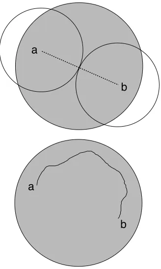
b
a
a
b
Figure 2. (a) Locating highest potential difference within the urbanized area (light grey—non-urbanized is white) between two pointaandbon the lattice using theFindMaxalgorithm. The urbanized “mass” within the two circle discs with centers inaandband radius12| a,b|determines the potential between the two points. (b) Successive iteration of theBuildRoadalgorithm generates a road betweenaandb.
decreasing manner as a function of the distance fromx.
The accessibilityAof a given transport node to a given point and is defined by
A(x,t)= 1
D(x,x−t). (3)
Thus accessibility of a transport node t to a given point x scales inversely as the den-sity/distance functionD; a given transport node’s accessibility to a fixed node goes down with distance from the node and with increased density of urbanized activity. Transportation over longer distances becomes more difficult through diffusion.
The available transportation betweenxandyvia existing roads is defined by
t(x,y)=
t∈T(x→y)
A(x,t) +
t∈T(y→x)
A(y,t), (4)
whereT(x→y) is the set of transport nodes aroundxdraining into the region around y
andT(y→x) is the set of nodes aroundydraining into the region aroundx, and Ais the accessibility of the transport nodes. More precisely
where R defines a road and the other symbols are defined above. T(y→x) is defined similarly. In words, the amount of transport structure between two points is the sum over local (in half-size regions around the two points) tranport nodes which access roads that link the two points, weighted by the accessibility of the two nodes.
The total potential betweenxandymay now be defined as
U(x,y)=D(x,d(x,y)/2)+D(y,d(x,y)/2)−t(x,y) (6) which expresses the demand for a road betweenxandy. It takes into account the weighted urbanization density in the regions around the two points and the availability of existing transportation infrastructure between them.
Note that an explicit (major) road between two points is sufficient to satisfy the travel demand. This means that we implicitly assume that each road has an infinite capacity and thus the only restriction on transportation between different points in the urban area is given by the diffusion to and from existing roads between the two points. This obvi-ous simplification may be taken into account by e.g. the introduction of a finite trans-portation capacity per transtrans-portation infrastructure unit (lattice site) combined with an integration of the transportation demand over the entire road, but it would complicate matters.
In these terms, the FindMax procedure finds (a,b)∈L×L that maximize U. See figure 2. The initiation of a new road is triggered by a transportation potential greater than a certain cut off,Uc.This numberUcis the maximal, possible distance of
transporta-tion without a major road. Again, we refer to transportatransporta-tion without major roads below this distance by diffusion (small local streets), in analogy to biological systems where e.g. the transport of nutrients at small scales occur through small capillary and through diffusion.
3.2. The BuildRoad procedure
This procedure recursively finds a close-to-minimal cost road between points chosen by
FindMax. See figure 3. We use a recursive process for choosing a close-to-optimal road.
Essentially, the road between points a and b is generated by evaluating the local cost of transportation nodes betweena andb for several points on the perpendicular through the midpoint of segmentab, accepting a minimal-cost nodec, and then re-executing the procedure betweenaandcand betweencandb. In other words, the road is built in segments from the middle out, picking the least-cost choice for the middle node of each segment. The recursion ends when the process reaches the level of resolution of the lattice (that is, distance betweend(a,b)≤√2).
Before we describe the actual structure of theBuildRoadprocedure, we will first for-mally define the cost function. To that end, let Pwiggle be a real 0≤Pwiggle≤1 and let
Pdensity=1−Pwiggle. Now let
Costa,b(c)=Pwiggle×[(d(a,c)+d(c,b))/d(a,b)]+Pdensity×D(c) (7)
densly populated (higher land prices) areas. The wiggle paramater Pwigglerepresents the
cost of geometric inefficiency in getting from one point to another, while its normalized complement,Pdensity, represents how costly building through dense areas is. The geometric
inefficiency of a given path between two points is measured by the ratio of the length of the path to the straight-line distance between the points. Activity density is measure by the same measure used in the potential functionU. The cost is thus the weighted aver-age of inefficiency and density, where the weights are represented by Pwiggle and Pdensity
respectively.
We can now define theBuildRoadprocedure. To choose a road betweenaandb(see figure 3):
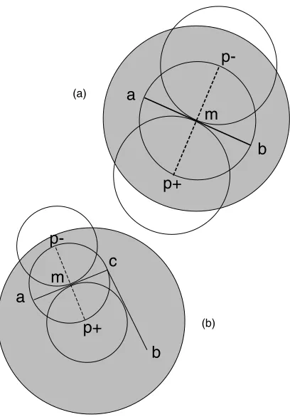
m
p+
p-b
a
m
c
a
b
p-p+
(a)(b)
Figure 3. Dynamics of theRoadBuildalgorithm. See text for more details. (a) The point paira,b, within the urbanized area which represents the highest potential is initially located byFindMax.mis the midpoint between aandbandp−andp+are located at distance1
ProcedureBuildRoad:
Letm, p+, and p−be the midpoint ofab, and the two intersections between a line perpendicular toabinmandC(m,|ab|) respectively.
l(a),l(b) :=2. Ifd(a,b)>√2, do:
Step 1:m:=midpoint along the vectorV = a,b.
l⊥:=line perpendicular toV passing throughm.
Step 2: Choose pointsp−andp+onl⊥whose distance frommisd(a,b)/2. Step 3: Evaluate the cost functionCosta,bat
1)m
2) p−
3) p+
Step 4: Letcbe the one which attains the minimum cost;l(c)=2.
Step 5: ExecuteBuildRoadfor:
1)a:=aandb:=cand 2)a:=candb:=b.
First, the recursion is initialized. Step 1 finds the appropriate line between the two points and its midpoint through geometric calculation. Step 2 finds the candidate points for road-building. Step 3 evaluates the cost function, the minimal value of which is picked in Step 4. The last step initiates the recursion on sub-segments.
Note that this road building dynamics can be executed on any data set, and can therefore be used independently in concert with any given land use generation dynamics that takes transportation infrastructure into account. Obviously the simple road building algorithm can also be exchanged with one of the classical corridor location algorithms to generate more realistic road structures.
4. Algorithmic complexity
The run-time complexity of the road growing dynamics is, for a circular lattice of ra-diusr with existing transport network of size T (number of transportation lattice points) given by
C(FindMax(r,T))+C(BuildRoad(r)), (8)
whereC( ) denotes run-time complexity. This is because theFindMaxandBuildRoad
procedures are on average independent and executed in sequence. Now, withU being the potential calculator as above, we estimate
This is because we calculate the potential function for each pair of non-tranportation nodes ((πr2−T)2pairs), so the complexity is the number of pairs times the complexity of the
potential calculation at each pair. We get that
C(U(r,T))=(2πr2+4r2T) (10)
because of the sequential independent structure ofUas a sum of “densities” minus a “exist-ing drainage” factor. The calculations go as the square of radius in the density component and asr2T in the existing drainage calculation since the density calculation requires summing over a circular area of average radiusr, and the drainage calculation requires calculating densities at each point in a drainage network of sizeT.
Finally,
C(BuildRoad)<3r (11)
because we calculate densities in circles of afixedradius (related to the paramaterα) an average of 3rtimes for each new road.
Thus the total algoritmic complexity is
(πr2−T)2(2πr2+4r2T)+3r, (12) which yields a run-time order asymtotic (for larger,T) of
r6(1+T)+T3. (13)
It is clear from the above that the major algoritmic complexity stems from the part of the dynamics that identifies the largest current transportation potential (FindMax). The actual road building algorithm (BuildRoad) is very simple (O(r)). A typical corridor location algorithm based on Dijkstra’s algorithm on the 2-D square lattice will have a run-time complexity ofO(r3) (Goodchild, 1977).
5. Growing roads
5.1. Stars and belt-ways
The growth of stars and belt-ways is mainly controlled by the balance between the cost of building roads through dense urbanized areas versus the cost of building longer and more winding roads. This balance is represented by the parametersPwiggleandPdensity=1−Pwiggle
(recall Eq. (7)). By varyingPwigglebetween 0 and 1 two significantly different roads growing
dynamics occur. For high values ofPwigglestars are formed and for moderate to low values
of Pwiggle belt-ways are formed if circular build areas (“cities”) without major roads are
used as seeding.
Figures 4 through 8 all use circular cities of diameter 11, 19, 25, and 49 lattice points. Note that at all size scales, variation ofPwigglealong its range significantly altered the qualitative
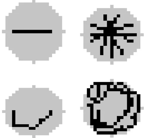
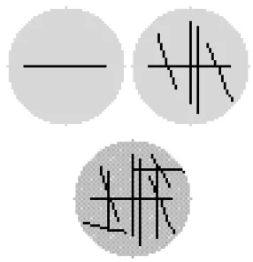
Figure 4. The evolution of a road network from an urbanized area of diameter 19 lattice sites initially without any main roads.Pwiggle=0.9 (upper figures): Roads after the first iteration (t=1) and after 6 iterations (t=6). Note the clear star shape of the generated transportation infrastructure. Pwiggle=0.4 (lower figures): Roads after the first iteration (t=1) and after 6 iterations (t=6). Note the clear belt-way structure of the generated transportation infrastructure.
of the transition from star to belt-way in the dynamics. The road network evolves multiple stars in the larger city as opposed to a single star in the smaller city. This is due to the local transportation diffusion being insufficient for transportation between the different “rays” of the central star due to the large distance between them. Diffusion is, however, sufficient for transportation into the rays of the central star as the distance between the rays is relatively small.
It is important to note that spatial symmetry of the resultant networks is not to be expected. For example, in those simulations with higherPwiggle, the first two steps tend to form a typical
“cross” formation. Once an initial “cross” formation is laid down, the next road often does not continue in the star-formation pattern that further symmetry of the cross formation would demand. That is because the “drainage” of the central area of the system after the first two iterations is very high, and the next few pairs of highest potential will not lie on a line traversing this higher-drainage central area.
5.2. Forced co-evolution between settlements roads
Figure 5. The evolution of a road network from an urbanized area of diameter 49 lattice sites initially without any main roads. First, fifth and tenth iterations are shown.Pwiggle=0.98 and the roads are straight and intra-city. This in the typical road growing dynamics for highPwigglevalues which is equivalent to high penalty for roads that “wiggle”. Compare with the small star in figure 4. The road growing dynamics is, as should be expected, in general dependent on the lattice size for fixedPwigglevalue. Note how the larger lattice allows more stars to coexist within the same city. See text for details.
evolution simulation. The initial condition is a small city (circle of radiusr) of urban-ized land with no major roads. Roads are then grown for some number of time steps and after that the previously non-urbanized areas within a circle of radius 2r are now urban-ized (that is non-urbanurban-ized land between 2randr), without disturbing already built roads and other build area. A second road-generation process is then applied without changing the parameters. This type of experiment is performed for the 25×25 and 50×50 lattices and city diameters 11 to 21 and 25 to 49, with various values of Pwiggle. See figures 7
and 8.
It is clear that these cities are more realistic looking that any of the previous “express-way retro-fitting” simulations. Again, independent of the lattice size for a rage of high
Pwiggleparameter values this two stage urban co-evolution of roads and settelments first
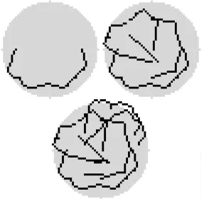
Figure 6. The evolution of a road network from an urbanized area of diameter 49 lattice sites initially without any main roads. First, fifth and ninth iterations are shown. ForPwiggle=0.40 the roads form belt-ways and reach out of the urbanized area. This is the qualitative road growing behavior for a wide range ofPwigglevalues until it approaches unity. Compare with the small belts in figure 4. As for the smaller lattice not all belt-ways connect as the potential (U) that drives the road growing dynamics diminishes as the local road density becomes very high. See text for details.
6. Discussion
6.1. More realistic road dynamics
Because we do not randomly select among multiple highest-potential pairs when multiples occur several apparent North/South and East/West biases are seen in the generated road data. This is because the algorithm chooses the first one with the highest potential, and because the FindMaxprocedure searches spatially always in the same order, this introduces an
apparently bias in the road patterns. Therefore, this bias is not an artifact of the algorithm, but rather a trivial artifact of the computer implementation.
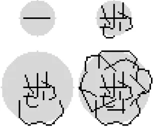
Figure 7. Forced co-evolution of settlements and roads on a small lattice. The evolution of a road network starts from an urbanized area initially without any main roads and withPwiggle=0.85. (a) After the first 3 iterations the urban system (diameter 11 lattice sites) has developed a clear star shaped transportation infrastructure. (b) At that time we externally impose a larger urbanized area around the original city center (lattice diameter 21) and continue to grow roads with the same value forPwiggle. At time 9 (after 6 addition iterations on the larger urban area keeping the original transportation infrastructure) a system of belt-ways have evolved around the center. Thus no parameter changes are necessary for the road growing dynamics if it is allowed to co-evolve with the settlement dynamics in a natural manner.
cost functions. The different parts of the belt-way are constructed at different steps of the simulations and since local transport diffusion occurs there is no local mechanism that makes sure that neighboring roads actually touch each other as planners would do in real cities. However, such an additional step in the algorithm could easily be implemented.
Perhaps the most serious problem with the current algorithm is that one important aspect of already existing transportation infrastructure is not taken into account as new roads are being built. As is, we subtract the existing roads between two “disks” aroundaandb. Recall Section 3.1. However, as we calculate the costs of building a connecting road betweenaand
bwe do not evaluate the alternative cost of partly connecting to existing roads that connects the disks aroundaandb. This is relatively simple modification that has to be implemented and tested. As mentioned earlier, one could also define a finite capacity for each road which can then be factored into the calculations (recall Section 3.1).
6.2. Where to go from here
The first question is how to define good, objective observables to determine algorithmically whether a road network is “realistic” or not. Obviously, the evolution of each real city consists of an accumulation of necessities and frozen accidents as all evolutionary processes do, and as such it is not obvious which generic features one can or should filter out. Batty and Longly (1994) and White et al. (1997) have analyzed urban form as well as certain parts of the urban transportation infrastructure along these lines using the fractal dimension as a major observable.
For the characteristic star versus belt-way features one possible, quantitative observable is the average ratio of road-length to intersection distance, where the ratio is taken over all roads. This quantity might be useful as long as only one of these road-features appears, but we have not made a systematic analysis of these issues yet.
Disaggregation is another important issue, which includes the high variability of the costs of real estate over a major metropolitan area as well as the difference in transportation generation and transportation requirements between for example housing on the one hand and commercial or industry on the other hand. The effects of such land-use disaggregations should be tested. For example, as it is now two “cost circle discs”, which are completely within the boundaries of the homogeneously build areas of the city, will represent the same cost (recall Sections 3.1 and 3.2). Perhaps the use of one of the corridor location algorithms is necessary to obtain sufficiently accurate transportation networks in a give geographic location.
guide retrofitting and improvements of existing transportation infrastructure within major metropolitan area.
The other (perhaps more obvious) application is as an a priori prediction tool, used in con-junction with existing land-use evolution algorithms to predict longer-term transport needs of urban growth into the future. Predictive algorithms (without co-evolving transportation) have been developed and refined for the last ten years by e.g. Clarke and co-workers at UC Santa Barbara (Clarke et al., 1997) and by White and co-workers at Memorial University in New Foundland (White et al., 1997) and latest in collaboration with Los Alamos (Andersson et al., 2002). These existing land-use evolution simulations require a pre-existing (projected) transportation network around which to evolve.
7. Conclusion
Varying the essential parameterPwiggle, which represents the balance of the additional cost
of building longer roads and the additional cost of building new roads through densly populated areas (higher land prices), the simulation generates global features of real urban transport systems:
1. The radiation of roads from the center of the city which generates a “star”, a feature of both planned and non-planned cities; (highPwigglevalues),
2. the homogeneous drainage in an irregular pattern, a feature of non-planned cities (low
Pwigglevalues), and
3. the formation of “belt-ways” around the center- and/or around the periphery of the city.
Low cost for building through dense areas favors star formation and high cost for building through dense areas favors belt-ways and more irregular network formation. For interme-diate values a transportation infrastructure can be generated which has both features. With a co-evolution of settlements together with roads more realism is present as an initial star-shaped transportation infrastructure irradiates out from the city center followed by the growth of belt-ways closer to the periphery as the urban settlements grow.
Acknowledgments
We are grateful for many enlightening discussions and suggestions from Roger White and Helen Couclelis as well as help in preparing some of the figures and proof reading by Tom Garrison and Claes Andersson. This work was financially supported by the Urban Security Initiative LDRD-DR and Science Based Programs at Los Alamos National Laboratory as well as by National Science Foundation (CMS-9902868).
References
Andersson, C., K. Lindgren, S. Rasmussen, and R. White. (2002). “Urban Growth Simulations from “First Prin-ciples.”Phys. Rev. E.66, 026204.
Batty, M. and P. Longley. (1994).Fractal Cities. New York: Academic Press.
Benenson, I. and J. Portugali. (1997). “Agent-Based Simulations of a City Dynamics in a GIS Environment.” COSIT501–502.
Benguigui, L. (1995). “A New Aggregation Model: Application to Town Growth.”PhysicaA 219, 13–26. Benguigui, L. and M. Daoud. (1995). “Is the Suburban Railway System a Fractal?”Geog. Analy.23, 362–368. Candau, J., S. Rasmussen, and K.C. Clarke. (2000). “A Coupled Cellular Automaton Model for Land Use/Cover
Dynamics.” InProc. 4th Int. Conf. on Integrating GIS and Environmental Modeling (GIS/EM4)Banff, Alberta Canada, Sept. 2–8.
Church, R.L., S.R. Loban, and K. Lombard. (1992). “An Interface for Exploring Spatial Alternatives for a Corridor Location Problem.”Comp. and Geosciences18(8), 1095–1105.
Clarke, K. and L. Gaydos. (1998). “Loose-Coupling a Cellular Automaton Model and GIS: Long-Term Urban Growth Prediction for San Francisco and Washington/Baltimore.”Int. J. Geographical Information Science 12(7), 699–714.
Clarke, K.C., S. Hoppen, and L. Gaydos. (1997). “A Self-Modifying Cellular Automaton Model of Historic Urbanization in the San Francisco Bay Area.”Env. and Plan.B 24(7), 247–261.
Couclelis, H. (1996). “From Cellular Automata to Urban Models: New Principles for Model Development and Implementation.”Artificial Worlds and Urban Studies, 165–190.
Ehlschlaeger, C.R. and A. Shortridge. (1996). “Modeling Elevation Uncertainty in Geographical Analyses.” In Proceedings of the International Symposium on Spatial Data Handling, 9B.15–9B.25.
Goodchild, M.F. (1977). “An Evaluation of Lattice Solutions to the Problem of Corridor Location.”Env, and Plan. A 9, 727–738.
Heiken, G., G. Valentine, M. Brown, S. Rasmussen, D. George, R. Greene, E. Jones, and C. Andersson. (2000). “Modeling Cities, The Los Alamos Urban Security Initiative.”Publ. Works Mang. and Policy4(3), 198–212. Lombard, K. and R.L. Church. (1993). “The Gateway Shortest Path Problem: Generating Alternative Routes for
a Corridor Location Problem.”Geographical Systems1, 25–45.
Makse, H.A., J.S. de Andrade, M. Batty, S. Havlin, and H.E. Stanley. (1998). “Modeling Urban Growth Patterns with Correlated Percolation.”Phys. Rev.E, 7059–7067.
Makse, H.A., S. Havlin, and H.E. Stanley. (1995). “Modelling Urban Growth Patterns.”Nature377, 608–612. Miller, H.J. (1999). “Beyond the Isotropic Plane: Towards a Geospatial Analysis.” UCSB Spatial Analysis
Workshop Papers.
Nagel, K., S. Rasmussen, and C. Barrett. (1997). “Network Traffic as a Self-Organized Critical Phenomenon.” In F. Schweitzer (ed.),Self-Organization of Complex Structures: From Individual to Collective Dynamics. Gordon and Breach, pp. 579–592.
Sanders, L., D. Pumain, and H. Mathian. (1997). “SIMPOP: A Multiagent System for the Study of Urbanism.” Env. and Plan.B 24, 287–305.
Schweitzer, F. (1997). “Active Walker Particles: Artificial Agents in Physics.” In L. Schimanski-Geier and T. Poschel (eds.),Stochastic Dynamics. Berlin: Springer Verlag, pp. 358–371.
Schweitzer, F., W. Ebelin, H. Rose, and O. Weiss. (1998). “Optimization of Road Networks Using Evolutionary Strategies.”Evol. Comp.5/4, 419–438.
Takeyama, M. (1996). “Geocellular: A General Platform for Dynamic Spatial Simulation.”Artificial Worlds and Urban Studies, 347–364.
http://transims.tsasa.lanl.gov
http://www.ees.lanl.gov/EES5/Urban Security/
White, R. and G. Engelen. (1997). “Multi-Scale Spatial Modelling of Self-Organizing Urban Systems.” In F. Schweitzer (ed.),Self-Organization of Complex Structures: From Individual to Collective Dynamics. pp. 519– 535.
White, R., G. Engelen, and I. Uljee. (1997). “The Use of Constrained Cellular Automata for High-Resolution Modeling of Urban Landscape Dynamics.”Env. and Plan.B 24, 323–343.
Wu, F. (1998). “SimLand: A Prototype to Simulate Land Conversion Through the Integrated GIS and CA with AHP-Derived Transition Rule.”Int. J. Geog. Info. Sci12, 63–82.
Xie, Y. (1996). A Generalized Model for Cellular Urban Dynamics.”Geographical Analysis28, 350–373. Yang, H. (1998). “Models and Algorithms for Road Network Design: A Review and Some New Developments.”