Inferring the depth distribution of catchability for
pelagic fishes and correcting for variations in the
depth of longline fishing gear
Peter Ward and Ransom A. Myers
Abstract:We introduce a new method that uses generalized linear mixed models to infer the depth distribution of pelagic fishes. It uses existing data from research surveys and observers on commercial vessels to estimate changes in catchability when longline fishing gear is lengthened to access deeper water. We infer the depth distribution of catchability for 37 fish species that are caught on pelagic longlines in the Pacific Ocean. We show how the estimates of catchability can be used to correct abundance indices for variations in longline depth. Our method facilitates the inclusion of data from early surveys in the time series of commercial catch rates used to estimate abundance. It also resolves inconsistencies in the time series caused by a rapid switch to deep longlining in the 1970s. The catchability distribution does not always match depth preferences derived from tracking studies. Therefore, depth preferences from tracking studies should not be used to correct abundance indices without additional information on feeding behavior.
Résumé :Nous présentons une nouvelle méthode qui utilise des modèles linéaires généralisés mixtes pour estimer la répartition des poissons pélagiques en fonction de la profondeur. La méthode exploite les données existantes
d’inventaires scientifiques et d’observations faites sur les navires commerciaux afin d’estimer les changements de capturabilité qui se produisent lorsqu’on allonge les palangres pour pêcher en eau plus profonde. Nous estimons la répartition de la capturabilité en fonction de la profondeur chez 37 espèces de poissons récoltés à la palangre pélagique dans le Pacifique. Nous démontrons comment les estimations de capturabilité peuvent servir à corriger les indices d’abondance en fonction des variations de la profondeur des palangres. Notre méthode facilite l’inclusion de données d’inventaires plus anciens dans la série chronologique de taux de capture commerciaux utilisée pour estimer
l’abondance. Elle permet aussi de résoudre les irrégularités dans la série chronologique causées par un passage rapide à la pêche à la palangre en profondeur durant les années 1970. La répartition de la capturabilité ne correspond pas toujours aux préférences de profondeur déterminées par les études qui traquent les poissons; il ne faut donc pas utiliser les préférences de profondeurs obtenues de ces études pour corriger les indices d’abondance s’il n’existe pas de rensei-gnements supplémentaires sur le comportement alimentaire.
[Traduit par la Rédaction] Ward and Myers 1142
Introduction
Recent analyses indicate that the state of the world’s pe-lagic fish stocks is much worse than previously believed. Most species of pelagic shark in the northwest Atlantic are now declining by about 10%·year–1(Baum et al. 2003). Ward and Myers (2005) found that the biomass of large sharks, tu-nas, and billfishes has fallen to one tenth of the level when pelagic longline fishing commenced in the tropical Pacific Ocean. Globally, the abundance of many large marine preda-tors is now less than 10% of the pre-exploitation level (Myers and Worm 2003).
The new perspective on the status of pelagic fishes is di-rectly linked to the recovery of historical data from longline surveys and commercial operations. However, critics have challenged conclusions based on those data, pointing to
un-certainties in using longline catch rates as indices of abun-dance. Longline fishing effort must be corrected or “stan-dardized” for variations in fishing practices and oceanographic conditions if abundance indices for early years are to be comparable with indices from recent years. The timing of longlining operations in relation to peak feed-ing periods is an example of a historical change in fishfeed-ing practices. Ward et al. (2004) found that changes in the tim-ing of longlintim-ing operations, which now have hooks avail-able during dusk as well as dawn, have resulted in the overestimation of abundance for many species in recent years.
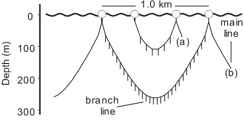
Another important historical change in longlining opera-tions is the depth range of the gear (Fig. 1), which is the topic of this article. Two methods have been used to account for changes in the depth distribution of longline hooks. One
62
Received 26 June 2004. Accepted 31 December 2004. Published on the NRC Research Press Web site at http://cjfas.nrc.ca on 31 May 2005.
J18197
P. Ward1,2and R.A. Myers. Department of Biology, Dalhousie University, Halifax, NS B3H 4J1, Canada.
1Corresponding author (e-mail: [email protected]).
method is to use generalized linear models to relate catches to longline depth and other explanatory variables. In most longline fisheries, however, a switch to deep gear was so rapid in the mid-1970s that there is inadequate temporal overlap to allow comparison of the performance of regular and deep gear (Suzuki et al. 1977). Takeuchi (2001) con-cluded that it was not possible to make reliable inferences about changes in abundance from historical longline catch and effort data.
The second method of correcting abundance indices for longline depth is to model the species’ preferred habitat. Oceanographic information (e.g., thermocline depth) is com-bined with information from tracking studies (e.g., Musyl et al. 2003) to estimate the species’ depth distribution in time and area strata (e.g., Hinton and Nakano1996; Bigelow et al. 2002). The habitat-based model is then combined with the inferred depth distribution of longline hooks to adjust the fishing effort for the species’ availability in each time–area stratum.
The previous methods required the estimation of an addi-tional parameter for each longlining operation included in the analysis. Consequently, estimates become increasingly biased as the sample size increases (Kiefer and Wolfowitz 1956). The generalized linear models used the proportions of catch at depth. However, the local abundance and gear con-figuration vary among longlining operations, causing further biases in the interpretation of the depth distribution derived from catch proportions. This article describes a new method that uses data from individual longline hooks to estimate rel-ative catchability at depth. The lack of an adequate statistical framework has previously precluded the use of individual hook data to derive statistically valid estimates of the depth distribution of catchability.
We use generalized linear mixed effect models (Wolfinger and O’Connell 1993), which have considerable advantages for estimating catchability at depth: (i) they allow for nonlin-ear relationships between independent variables and the dependent variable (mean catch), (ii) a variety of error distri-butions (e.g., Poisson) can be modeled, and (iii) they allow local abundance to be a random variable, providing
statisti-cally consistent estimates with improved accuracy (Robin-son 1991).
Variations in fishing gear and oceanographic conditions affect catchability, the part of a stock that is caught by a de-fined unit of fishing effort. The catchability coefficient q re-lates catch C to the species’ local abundance N and the amount of fishing effortE:
(1) C = qEN
A reliable estimate of catchability is therefore necessary to estimate abundance from catch and effort data (Murphy 1960). Catches are the product of catchability, local abun-dance, and fishing effort. For longline gear, fishing effort is often measured as the number of longline hooks available at each depth. Our approach is to first estimate the depth distri-bution of catchability independent of availability. We then take availability into account by adjusting the number of hooks at each depth by the estimated catchability.
Materials and methods
Data
We analyzed data collected by scientists involved in a re-search survey and by observers on commercial vessels using pelagic longlines. The data included gear dimensions for each longlining operation, which we used to estimate the maximum settled depth of each hook deployed. The scien-tists and observers also reported a unique identifier, a se-quential number, for each longline hook. Combined with the gear dimensions, the individual hook data were used to esti-mate the depth at which each animal was caught.
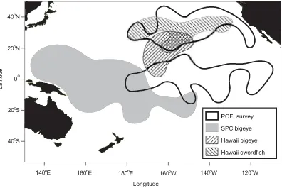
We combined three data sets. The US Pacific Oceanic Fisheries Investigations conducted 1157 longlining opera-tions in an area of the Pacific Ocean bounded by 175°E– 115°W and 12°S–44°N during 1950–1958 (Fig. 2). Survey longliners used fishing gear and techniques adopted from Ja-pan (Murphy and Shomura 1972). They typically deployed longlines at dawn each day and retrieved in the afternoon. They usually attached six hooks between each pair of floats, amounting to about 240 hooks in each daily longlining oper-ation. The maximum settled depth of the hooks ranged from 18 to 103 m (unless otherwise indicated, all hook depths were estimated from the catenary formula reduced by 25% for the effects of currents). The survey longliners occasion-ally deployed longlines at night and deep longlines with up to 21 hooks between floats (18–144 m). They mostly used sardines (Sardinellaspp.) as bait but also experimented with saury (Scomberesox spp.), squids (Illex spp.), and various other baits.
The second data set was from US National Marine Fish-eries Service observers placed on commercial longliners in the Pacific Ocean during 1994–2002. The data consisted of 8037 daily longlining operations in an area bounded by 5°N–40°N and 174°E–134°W. The longliners targeted broadbill swordfish (Xiphias gladius) or tunas, specifically bigeye tuna (Thunnus obesus) and yellowfin tuna (Thunnus albacares), for domestic fresh-fish markets. To catch tunas in tropical waters, they deployed deep longlines with sar-dines as bait during the day with about 28 hooks between floats (40–230 m). To catch swordfish in temperate waters, Fig. 1.Configuration of (a) a regular longline with six hooks
they deployed shallower longlines (39–121 m) with shortfin squid (Illex illecebrosus) as bait at night.
The Secretariat of the Pacific Community assembled the third data set from data collected by observers placed on commercial longliners during 1992–2002. The data consisted of 1813 longlining operations in an area of the Pacific Ocean bounded by 27°S–12°N and 138°E–172°W. Most of the longliners targeted bigeye tuna during the day with deep longlines consisting of about 30 hooks between floats (33– 267 m). They used saury, sardines, or squids as bait.
The longliners used similar fishing gear, e.g., comparable hook sizes and wire leaders to connect hooks to branch lines. The longliners monitored by US National Marine Fisheries Service and Secretariat of the Pacific Community observers deployed monofilament-nylon branch lines, whereas the survey longliners used rope gear. The next section de-scribes the random effects model that are used to account for variations in local abundance and catches among longlining operations. It was included to reduce the effects on catchability of variations in bait and fishing gear among longline operations.
Observers and survey scientists identified the species and recorded the hook number for each animal caught. Occa-sionally, they did not identify animals to the species level, so that species were combined into species groups. For brevity, we use the term species group to refer to individual species as well as species groups. The US National Marine Fisheries Service observers did not record the hook number for spe-cies groups other than tunas, billfishes, and sharks.
We assumed that the mainline formed a catenary curve be-tween each pair of floats and estimated the depth of each
hook by applying the formula presented by Suzuki et al. (1977) to longline dimensions reported for each operation. We assumed that the shape of the catenary curve (and there-fore the corresponding depth of hooks) did not systemati-cally vary along each longline or during each longline operation. Observed depths and predicted depths are known to vary, with ocean currents and wind having the most im-portant influence on hook depth. Bigelow et al. (2002) esti-mated that hook numbers 3 and 10 of longline gear with 13 hooks between floats shoaled by about 20% when subjected to a current velocity of 0.4 m·s–1. To represent shoaling of longlines in our study area, we reduced all depths predicted by the catenary formula by 25%. The data were then binned into 40-m depth categories ranging from 0–40 to 480–520 m.
We estimated catchability distributions separately for day and night operations. Most day operations commenced at dawn (the median deployment time was 0705 (local) with 50% beginning between 0520 and 0747). Night operations often started at dusk (median time of 1817 with 50% be-tween 1711 and 1930). We analyzed a total of 3155 night operations (13 679 animals) and 7852 day operations (32 046 animals) (Table 1).
Models
only a small proportion of the hooks are occupied by a spe-cies group, e.g., the mean percentage of hooks occupied by one of the most abundant species, yellowfin tuna, was 1.7% ± 4.1% SD.
For each species group, the model predicts the mean catch µi,Dusing a log link:
(2) log(µi D, )= λi+γ1D+γ2D2 +γ3D3+log(Hi D, )
where λi and γj are parameters estimated for each species group and the offsetHi,Dis the number of hooksHdeployed
at depthDof longlining operationi. Our method includes a random effects model that accounts for variations in the lo-cal abundance of each species. We assumed that the log abundance of the species group, when it is encountered, fol-lowed the random effects distribution, which we assumed to be a normal distribution,
λi~ N( ,µ σ2)
The regression coefficients γj in eq. 2 describe how catchability changes with depth (µ represents catch, H is
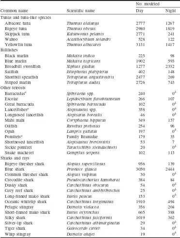
No. modeled
Common name Scientific name Day Night
Tunas and tuna-like species
Albacore tuna Thunnus alalunga 2777 1267
Bigeye tuna Thunnus obesus 2980 1819
Skipjack tuna Katsuwonus pelamis 2771 241
Wahoo Acanthocybium solandri 528 122
Yellowfin tuna Thunnus albacares 3131 1417
Billfishes
Black marlin Makaira indica 225 98
Blue marlin Makaira nigricans 1902 593
Broadbill swordfish Xiphias gladius 1277 2332
Sailfish Istiophorus platypterus 402 148
Shortbill spearfish Tetrapturus angustirostris 2477 269
Striped marlin Tetrapturus audax 2726 743
Other teleosts
Barracudasa Sphyraenaspp. 240 0b
Escolar Lepidocybium flavobrunneum 266 107
Great barracuda Sphyraena barracuda 102 0b
Lancetfishesa Alepisaurusspp. 358 0b
Longnosed lancetfish Alepisarus borealis 46 0b
Mahi mahi Coryphaena hippurus 349 157
Oilfish Ruvettus pretiosus 254 96
Opah Lampris guttatus 197 0b
Pomfretsa Family Bramidae 179 35
Shortnosed lancetfish Alepisaurus brevirostris 53 7
Sickle pomfret Taractichthys steindachneri 20 0b
Snake mackerel Gempylus serpens 102 113
Sharks and rays
Bigeye thresher shark Alopias superciliosus 956 139
Blue shark Prionace glauca 3050 2444
Common thresher shark Alopias vulpinus 30 0b
Crocodile shark Pseudocarcharias kamoharai 384 84
Dusky shark Carcharhinus obscurus 54 0b
Grey reef shark Carcharhinus amblyrhynchos 25 0b
Long-finned mako shark Isurus paucus 153 0b
Oceanic whitetip shark Carcharhinus longimanus 1910 494
Pelagic stingray Dasyatis violacea 356 204
Short-finned mako shark Isurus oxyrinchus 665 388
Silky shark Carcharhinus falciformis 1019 362
Silver-tip shark Carcharhinus albimarginatus 29 0b
Tiger shark Galeocerdo cuvier 34 0b
Whip stingray Dasyatis akajei 19 0b
aOccasionally, observers did not identify animals to the species level. Consequently, we modeled data for
species groups (e.g., barracudas (Sphyraenaspp.)) separately to data for identified species (e.g., great barracuda (Sphyraena barracuda)).
bInsufficient numbers caught to allow reliable parameter estimation.
fishing effort, and theγjparameters represent catchability in eq. 1). For each species group, we sequentially tested in-creasingly complex functional forms of eq. 2 to find the most appropriate model. We initially fitted eq. 2 with γ1 = γ2=γ3= 0 and then tested the model in which we estimated γ1 while constraining the quadratic and cubic parameters to zero. We sequentially added otherγjparameters until the in-crease in the fit of the model was not significant as judged by a likelihood ratio test. The cubic model adequately de-scribed most of the variation in depth; including additional terms had very little effect on parameter estimates.
We then used parameter estimates, denoted by the “hat” symbol, from eq. 2 to estimate the catchability of each spe-cies group as a function of hook depthD (metres):
f D( )=exp(α +γ$1D+γ$2D2 + γ$ D
3 3)
where α is chosen such that the mean of f(D) equals one over the depth range considered. We refer to these standard-ized f(D) as the depth distribution of catchability or simply the catchability distribution.
Correcting abundance indices for depth effects
To correct abundance indices for variations in longline depth, we can apply our estimates to data where gear dimen-sions are known for each operation. They can also be used to correct indices for changes in catchability when only the proportion of gear configurations is known. In almost all cases, the longline configuration is identical between floats and symmetrical. Therefore, the number of depths k that needs to be considered for each gear configuration is half the number of hooks between floats. We then estimatedqg, which is the average catchability of the species group for gear con-figurationg: each year, the catchability averaged over all gear configura-tions is
qy Py gq
g g
=
∑
,where Py,g is the proportion of longlining operations using gear configuration g in year y. For each species group, we standardized the average catchabilityqyby dividing it by its value in the first year of the time series.
We illustrate the effect of the depth correction by applying it to a time series of annual catch rates for Japan’s longline fleet operating in the southern Atlantic Ocean. Estimation of the average annual catchability used the depth distribution of catchability combined with changes in gear configurations reported by Suzuki et al. (1977) and Uozumi and Nakano (1996). For each year, we divided the species’ catch rate by our estimate of its average catchability for all gear configu-rations qy. We then standardized the estimate by dividing it by the average catchability in 1975 (the first year of the time series).
Results and discussion
Precision of depth estimates
The application of our estimates of the depth distribution of catchability should not be affected by uncertainty over the depths of longline hooks estimated by the catenary formula. It is true that observed depths (obtained using depth sensors) and predicted depths often differ. The weight of the longline causes a gradual shortening in the distance between floats during the operation. Consequently, longline hooks may sink to deeper depths than those predicted by the catenary for-mula. At the same time, wind and current sheer may cause hooks to rise towards the surface or “shoal” (Hanamoto 1987; Mizuno et al. 1999). However, we contacted several observ-ers and longline fishobserv-ers who pointed out that commercial fishers adjust their fishing practices to maximize the avail-ability of longline hooks to target species, such as deep-dwelling bigeye tuna. Since the 1980s, many longliners have used Doppler current profilers to monitor the velocity and direction of subsurface currents. Most fishers minimize shoaling by deploying their longline in the same direction as prevailing currents. Furthermore, the predicted depth distri-butions of the hooks are surrogates for their true, but un-known, depth distributions. Our approach does not require accurate depth estimates because exactly the same methods and corrections that we used to estimate depth for our mod-els can be applied to the longline data that are being corrected. By contrast, the depth estimates from tracking studies that are used in habitat-based models are not calibrated against longline depth.
Various factors may influence the depth distribution of catchability derived from observer data, e.g., spatial and sea-sonal variations in wind, currents and thermal structure and differences in fishing practices and gear among fleets. Our presentation of one night and one day distribution for each species should not preclude further investigation of the im-portance of those influences on depth distributions.
Ecological groups
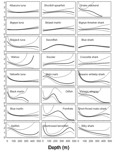
We derived reliable estimates of the depth distribution of catchability for 37 species groups over a depth range of 18– 512 m for day operations (Fig. 3) and for 24 species groups over 28–504 m for night operations (Fig. 4) (Appendix A provides parameter estimates for each species). The species groups show considerable variability in the distribution of catchability. The distributions indicate at least three distinct ecological groups, which should be considered separately in ecosystem models: epipelagic species that feed in surface waters (<200 m) during the day, wide-ranging pelagic spe-cies whose catchability does not vary over the observed depth range, and mesopelagic species that feed at intermediate and deep depths (>200 m) by day and then range more widely at night. Few species groups show high catchability at interme-diate depths (200–400 m).
The epipelagic group includes oceanic whitetip shark (Carcharhinus longimanus), dusky shark (Carcharhinus obscurus), skipjack tuna (Katsuwonus pelamis), mahi mahi (Coryphaena hippurus), wahoo (Acanthocybium solandri), and all billfishes except swordfish. They were most often caught in surface waters above the thermocline (about 140 m in the tropical Pacific Ocean) during the day (Fig. 3). How-ever, some were also caught on deep hooks. This is probably because animals may be caught when “deep” hooks pass through surface waters during longline deployment and re-trieval (Boggs 1992).
Diel variation
Comparisons of catchability for day and night operations (Figs. 3 and 4) reveal patterns of diel variation among the mesopelagic species that probably represent vertical migra-tion. The catchability of bigeye tuna, for example, increases with depth during the day, whereas it shows a much more uniform distribution at night. Our interpretation is that visi-bility is critical to the vertical distribution of large predators like bigeye tuna in the open ocean. They have several
physi-ological adaptations, such as large eyes, that provide acute vision and allow them to hunt at low light levels (Pereira 1996). They feed below the sunlit zone during the day where they can avoid detection by their prey. At night, they range more widely because the ocean is almost uniformly dark. The distributions of other large predators indicate patterns of vertical migration that are similar to that of bigeye tuna, e.g., albacore tuna (Thunnus alalunga), escolar (Lepidocybium flavobrunneum), and bigeye thresher shark (Alopias super-ciliosus).
Visibility is also critical for predator avoidance by small species, such as snake mackerel (Gempylus serpens), which are the prey of large tunas, billfishes, and sharks (Kitchell et al. 1999; Rosas-Alayola et al. 2002). These small species concentrate at deep depths, below the sunlit zone during the day, where they can avoid their predators. At night, they venture into surface waters. Several epipelagic species show the opposite pattern, concentrating in surface waters during the day and then ranging more widely at night, e.g., shortbill spearfish (Tetrapturus angustirostris) and striped marlin (Tetrapturus audax).
The depth distribution of catchability does not change markedly between day and night for several species, e.g., skipjack tuna, mahi mahi, and sailfish (Istiophorus pla-typterus). These epipelagic species are most abundant in sur-face waters. Hook-timer experiments (e.g., Boggs 1992) confirm that they are often caught in surface waters, particu-larly during longline deployment and retrieval. Night long-lining operations caught fewer species groups than day operations, and the night depth distributions for several epipelagic species are poorly estimated compared with the estimates of their daytime distributions. This is partly due to differences in sample sizes (we analyzed 3155 night opera-tions compared with 7852 day operaopera-tions). The poor esti-mates of night distributions might also be related to diel
variations in feeding activity. Stomach content analyses indicate reduced feeding activity among many epipelagic species at night. Analyses of the stomach contents of sailfish by Rosas-Alayola et al. (2002), for example, show that this species feeds mainly in surface waters during the day.
Comparison with tracking studies
several days. Recent studies using archival tags (e.g., Musyl et al. 2003) have allowed the depth preferences of animals to be estimated over longer periods, thereby providing a more complete understanding of their behavior.
Our estimates of catchability distributions from longlining operations provide a good match to the tracking data in sev-eral cases (Fig. 5). For example, tagged black marlin (Makaira indica) spent most of the day in surface waters, which matches the catchability distribution (Fig. 5g). For bigeye tuna, however, the tracking data show patterns differ-ent from the catchability distribution (Figs. 5a and 5b). The
inconsistencies between catchability distributions and depth preferences may be due to the small numbers of animals tracked or differences in behavior and oceanographic condi-tions between our broad study area and the areas where the animals were tracked. Eight of the yellowfin tuna tracked by Holland et al. (1990a) (Fig. 5c), for example, were associated with fish-aggregating devices. Those animals were found to be-have quite differently from yellowfin tuna in the open ocean.
The inconsistencies between the depth distribution of catchability and depth preferences derived from tracking studies might also reflect a mismatch between the estimated
Species Device
No. of animals
Time at
liberty Location Reference
Bigeye tuna Archival tags 4 9–76 days Southwestern Hawaii Musyl et al. 2003
Yellowfin tuna Ultrasonic transmitters 11 5 h – 6 days Hawaii Holland et al. 1990a
Blue marlin Ultrasonic transmitters 5 24–42 h Hawaii Holland et al. 1990b
Black marlin Ultrasonic transmitters 4 18–24 h Northeastern Australia Pepperell and Davis 1999 Table 2.Details of tracking data used to estimate the proportion of time spent at each depth.
depth of longline hooks and tracking depths or differential vulnerability to longline fishing gear. It is quite possible for a species to be abundant at depths where they have a re-duced vulnerability to the gear. For example, bigeye tuna might be present in surface waters during the day but not caught on longline hooks there because they are not feeding or cannot detect the baits. This is not of concern because we intend the estimates of catchability to be used to correct abundance indices derived from longline data. However, the mismatch between catches on longline hooks and the spe-cies’ depth preference is a flaw in habitat-based models that are solely based on tracking data. Tracking data show an an-imal’s depth preference, which may not always match the species’ vulnerability to longline fishing gear. From an anal-ysis of simulated data for blue marlin (Makaira nigricans), Goodyear (2003) concluded that the propensity of the spe-cies to take longline baits and the actual depth profile of the fishing gear strongly influenced habitat-based model esti-mates of abundance. The development of statistical habitat-based models, which fit observed catches (Hinton and Maunder 2003), may help to correct for differences between depth preferences and vulnerability.
An alternative to our approach is to use hook-timers that record the time and depth when each animal was caught (e.g., Boggs 1992). However, a very large number of hook-timer experiments are required to derive reliable estimates of depth preference. For example, Matsumoto et al. (2001) ana-lyzed over 300 longlining operations, each deploying 10– 163 hook-timers. However, that number of experiments was not large enough to obtain reliable estimates of depth prefer-ence.
Environmental constraints on depth distribution
The tracking studies show that environmental conditions set broad limits to the vertical distribution of each species. Those limits will also apply to the depth distribution of catchability. For example, Brill et al. (1993) concluded that sharp gradients in water temperature between the mixed layer and deeper waters represented a barrier to vertical mi-grations of striped marlin near Hawaii. Other conditions, such as oxygen concentration, are also known to limit the vertical distribution of pelagic fishes (Hanamoto 1987). The efficacy of those thresholds will vary seasonally, spa-tially, among species, and with body size (Dagorn et al. 2000). Caution is required in applying our estimates of catchability distributions to regions outside the study area. For example, the shallow thermocline in the tropical east-ern Pacific Ocean results in very low catch rates of striped marlin on longline hooks below about 100 m (Matsumoto and Miyabe 2002). By contrast, our estimates indicate an average level of catchability for striped marlin below 100 m (Figs. 3 and 4).
Further work is required to determine whether our esti-mates can be applied to other regions. Several organizations hold hook-level data that we could not access, e.g., data col-lected by British observers on longliners in the Indian Ocean and surveys by Japan’s National Research Institute of Far Seas Fisheries. Such data sets should be used to test the hy-pothesis that the shape of a species’ catchability distribution does not vary among regions or seasons but is compressed or extended by local conditions that limit the species’ depth
range. Data were not available to model the effects of body size on the depth distribution of each species, but we expect further work to show that larger animals generally have a wider depth range.
Correcting longline catch rates
There are two ways that our estimates of the depth distri-bution of catchability can be used to improve estimates of abundance. First, correction factors can be applied to operation-level data where gear dimensions and the number of hooks between floats are known for each operation. Such data exist for a large number of longline surveys conducted before commercial fishing commenced (e.g., Wathne 1959) and for more recent research cruises and monitoring pro-grams. Ward and Myers (2005) illustrated how the correc-tion factors can adjust abundance indices derived from longline surveys in the 1950s and commercial operations in the 1990s.
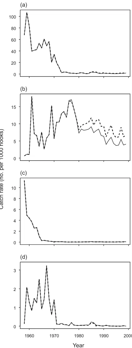
The second application of our estimates is to correct abun-dance indices for changes in depth when only the proportion of gear configurations is known. Japan’s longliners rapidly switched from regular longlining (<120 m) to deep long-lining (deepest hooks ranging beyond 120 m) in the Atlantic Ocean in the late 1970s (Fig. 6a). The introduction of deep longlining had virtually no effect on the catchability of yellowfin tuna and swordfish (Figs. 6b and 6c). Catchability declined for marlins and sailfish but increased by 60% for bigeye tuna and by 40% for albacore tuna. While these changes warrant their inclusion in assessment models, they are less than those estimated by the early nonstatistical habitat-based models (e.g., Hinton and Nakano 1996).
The application of our depth correction to annual catch rates of longliners in the southern Atlantic Ocean illustrates how variations in gear configurations can affect estimates of abundance. We have previously advised caution in applying our estimates of catchability to regions outside the study area; this application to the southern Atlantic Ocean is only intended to illustrate how the estimates can be used. The use of longline catch rates as indices of abundance is also sub-ject to debate (R.A. Myers and A.M. Edwards, unpublished data). The introduction of deep longlines resulted in the overestimation of bigeye tuna abundance but had a relatively small effect on abundance indices for other species (Fig. 7). In absolute terms, the effect is small on estimates of blue marlin, sailfish, and albacore tuna because of the significant decline in the abundance of those species well before the switch to deep longlining (Myers and Worm 2003). Further-more, deep hooks take about 30 min to move through shal-low and intermediate depths during longline deployment and retrieval. Consequently, catches are smeared over a range of depths (Boggs 1992).
they now constitute only a small part of the pelagic fish community available to longline fishing gear.
In summary, we have demonstrated a method where abun-dance indices derived from longline catch rates can be
cor-rected for historical variations in the depth range of the fish-ing gear. The method is relatively simple to apply and uses existing data that previously lacked the appropriate statisti-cal framework for analysis. It can be applied to bycatch spe-Fig. 6.Historical variations in gear configurations and catchability.
(a) Number of hooks between floats deployed by Japan’s longline fleet in the tropical Atlantic Ocean (modified from Yokawa and Uozumi (2001)). Hooks between floats is a rough indicator of longline depth range (for these operations, six hooks between floats produces a depth range of about 50–150 m compared with 50–300 m for a configuration with 14 hooks between floats). (b) Estimated change in average catchability over all gear configu-rationsqy used by the tropical Atlantic fleet relative to the 1975 gear configuration. (c) Change in the depth distribution of catchabilityqgrelative to the gear configuration with three hooks between floats for six species taken by the tropical Atlantic fleet.
cies that have not been the subject of tracking studies and it accommodates early data where only approximate gear char-acteristics are known and detailed oceanographic data are not available. Our method also eliminates the confounding in other statistical methods caused by the rapid switch to deep longline gear in the 1970s. Thus, we reject the claim by Takeuchi (2001) that abundance indices cannot be corrected for historical changes in the depth of longline hooks.
Longliners have maintained catch rates of target species by improving the efficiency of their fishing gear (Stone and Dixon 2001), increasing soak time, ensuring that hooks are available at peak feeding periods (Ward et al. 2004), and by extending the geographical limits of fishing grounds (Myers and Worm 2003). In the 1970s, they also began to exploit a much greater depth range. Our analyses show that deep longlining has resulted in the underestimation of the abun-dance of several epipelagic species (e.g., sailfish). However, it has resulted in the overestimation of the abundance of sev-eral pelagic species, including target species like bigeye tuna. Those large predators not only support valuable fishing in-dustries, they have unique ecological roles, influencing the diversity and abundance of lower trophic levels.
Acknowledgments
The work is part of a larger project on pelagic longlining that was initiated and sponsored by the Pew Charitable Trusts. We also thank the Pelagic Fisheries Research Pro-gram, the Natural Sciences and Engineering Research Coun-cil of Canada, and the Future of Marine Animal Populations project of the Sloan Foundation Census of Marine Life for financial support. Tim Davis, Brent Miyamoto, Mike Musyl, Tom Swenarton, and Peter Williams provided data and infor-mation on the fisheries. Wade Blanchard and Darren Swan provided technical advice. Two reviewers provided com-ments on the manuscript.
References
Baum, J.K., Myers, R.A., Kehler, D.G., Worm, B., Harley, S.J., and Doherty, P.A. 2003. Collapse and conservation of shark popula-tions in the northwest Atlantic. Science (Wash., D.C.), 299: 389–392.
Bigelow, K.A., Hampton, J., and Miyabe, N. 2002. Application of a habitat-based model to estimate effective longline fishing ef-fort and relative abundance of Pacific bigeye tuna (Thunnus obesus). Fish. Oceanogr.11: 143–155.
Boggs, C.H. 1992. Depth, capture time, and hooked longevity of longline-caught pelagic fish: timing bites of fish with chips. Fish. Bull.90: 642–658.
Brill, R.W., Holts, D.B., Chang, R., Sullivan, S., Dewar, H., and Carey, F.G. 1993. Vertical and horizontal movements of striped marlin (Tetrapturus audax) near the Hawaiian Islands, deter-mined by ultrasonic telemetry, with simultaneous measurement of oceanic currents. Mar. Biol.117: 567–574.
Carey, F.G., and Robison, B.H. 1981. Daily patterns in the daily activity patterns of swordfish, Xiphias gladius, observed by acoustic telemetry. Fish. Bull. 79: 277–291.
Carey, F.G., and Scharold, J. 1990. Movements of blue sharks (Prionace glauca) in depth and course. Mar. Biol.106: 329–342. Dagorn, L., Bach, P., and Josse, E. 2000. Movement patterns of
large bigeye tuna (Thunnus obesus) in the open ocean, deter-mined using ultrasonic telemetry. Mar. Biol.136: 361–371.
Goodyear, C.P. 2003. Tests of the robustness of habitat-standardized abundance indices using simulated blue marlin catch-effort data. Mar. Freshw. Res.54: 369–381.
Hanamoto, E. 1987. Effect of oceanographic environment on bigeye tuna distribution. Bull. Jpn. Soc. Fish. Oceanogr.51: 203–216. Hinton, M.G., and Maunder, M.N. 2003. Methods for
standardiz-ing cpue and how to select among them. ICCAT Coll. Vol. Sci. Pap. SCRS/2003/034.
Hinton, M.G., and Nakano, H. 1996. Standardizing catch and effort statistics using physiological, ecological, or behavioural con-straints and environmental data, with an application to blue mar-lin (Makaira nigricans) catch and effort data from the Japanese longline fisheries in the Pacific. Inter-Am. Trop. Tuna Comm. Bull.21: 169–200.
Holland, K., Brill, R., and Chang, R. 1990a. Horizontal and verti-cal movements of yellowfin and bigeye tuna associated with fish aggregating devices. Fish. Bull.88: 493–507.
Holland, K., Brill, R., and Chang, R. 1990b. Horizontal and verti-cal movements of Pacific blue marlin captured and released us-ing sportfishus-ing gear. Fish. Bull.88: 397–402.
Kiefer, J., and Wolfowitz, J. 1956. Consistency of the maximum likelihood estimator in the presence of infinitely many incidental parameters. Ann. Math. Stat.27: 887–906.
Kitchell, J.F., Boggs, C., He, P., and Walters, C.J. 1999. Keystone predators in the central Pacific.InEcosystem approaches for fish-eries management.Edited by J.N. Ianelli. University of Alaska Sea Grant, Fairbanks, Alaska. pp. 665–684.
Matsumoto, T., and Miyabe, H.S.N. 2002. Report of observer pro-gram for Japanese tuna longline fishery in the Atlantic Ocean from September 2001 to March 2002. Tech. Rep. SCRS/02/140, ICCAT Coll. Vol. Sci. Pap.
Matsumoto, T., Uosumi, Y., Uosaki, K., and Okazaki, M. 2001. Preliminary review of billfish hooking depth measured by small bathythermograph systems attached to longline gear.In Report of the Fourth ICCAT Billfish Workshop, Miami, Fla., 18– 28 July 2000). International Commission for the Conservation of Atlantic Tunas, Madrid. pp. 337–344.
Mizuno, K., Okazaki, M., Nakano, H., and Okamura, H. 1999. Es-timating the underwater shape of tuna longlines with micro-bathythermographs. Inter-Am. Trop. Tuna Comm. Spec. Rep. No. 21.
Murphy, G.I. 1960. Estimating abundance from longline catches. J. Fish. Res. Board Can.17: 33–40.
Murphy, G.I., and Shomura, R.S. 1972. Pre-exploitation abundance of tunas in the equatorial central Pacific. Fish. Bull.70: 875–913. Musyl, M.K., Brill, R.W., Boggs, C.H., Curran, D.S., Kazama,
T.K., and Seki, M.P. 2003. Vertical movements of bigeye tuna (Thunnus obesus) associated with islands, buoys, and seamounts near the main Hawaiian Islands from archival tagging data. Fish. Oceanogr.12: 152–169.
Myers, R.A., and Worm, B. 2003. Rapid worldwide depletion of predatory fish communities. Nature (Lond.), 423: 281–283. Pepperell, J., and Davis, T. 1999. Post-release behaviour of black
marlin, Makaira indica, caught off the Great Barrier Reef with sportfishing gear. Mar. Biol. 135: 369–380.
Pereira, J.G. 1996. Bigeye tuna: access to deep waters.InFirst World Meeting on Bigeye Tuna, 11–15 November 1996. Edited by R.B. Deriso, W.H. Bayliff, and N.J. Webb. Inter-American Tropical Tuna Commission, La Jolla, Calif. pp. 243–249.
Robinson, G.K. 1991. That BLUP is a good thing: the estimation of random effects. Stat. Sci.6: 15–51.
sailfish (Istiophorus platypterus) from the southern Gulf of Califor-nia, Mexico. Fish. Res. (Amst.),57: 185–195.
Stone, H.H., and Dixon, L.K. 2001. A comparison of catches of swordfish,Xiphias gladius, and other pelagic species from Ca-nadian longline gear with alternating monofilament and multi-filament nylon gangions. Fish. Bull.99: 210–216.
Suzuki, Z., Warashina, Y., and Kishidam, M. 1977. The compari-son of catches by regular and deep tuna longline gears in the western and central equatorial Pacific. Bull. Far Seas Fish. Res. Lab.15: 51–89.
Takeuchi, Y. 2001. Is historically available hooks-per-basket infor-mation enough to standardize actual hooks-per-basket effects on cpue? Preliminary simulation approach. ICCAT Coll. Vol. Sci. Pap.53: 356–364.
Uozumi, Y., and Nakano, H. 1996. A historical review of Japanese longline fishery and billfish catches in the Atlantic Ocean. In Collective volume of scientific papers. Report of the second
ICCAT Billfish Workshop. International Commission for the Conservation of Atlantic Tunas, Madrid. pp. 233–243. Ward, P., and Myers, R.A. 2005. Shifts in open-ocean fish
commu-nities coinciding with the commencement of commercial fish-ing. Ecology, 86(4): 835–847.
Ward, P., Myers, R.A., and Blanchard, W. 2004. Fish lost at sea: the effect of soak time and timing on pelagic longline catches. Fish. Bull.102: 179–195.
Wathne, F. 1959. Summary report of exploratory longline fishing for tuna in Gulf of Mexico and Caribbean Sea, 1954–1957. Commer. Fish. Rev.21: 1–26.
Wolfinger, R., and O’Connell, M. 1993. Generalized linear mixed models: a pseudo-likelihood approach. J. Stat. Comput. Sim.48: 233–243.
Yokawa, K., and Uozumi, Y. 2001. Analysis of operation pattern of Japanese longliners in the tropical Atlantic Ocean and their blue marlin catch. ICCAT Coll. Vol. Sci. Pap.53: 318–336.
Appendix A. Estimates of depth distribution parameters derived from pelagic longline data.
We used generalized linear mixed effect models with a Poisson distribution to model the mean catchµof each species or species group in longline operation iat depth D. The model predicted the mean catch using a log link:log(µi D, )= λi+γiD+γ2D2+γ3D3+log(Hi D, )
where the “offset”Hi,Dis the number of hooks deployed at depthDin longline operationi, andλiis the random effects distri-bution for the species in operationi(we assumed that the log abundance of the species encountered by each operation follows a normal distribution). The regression coefficients γjdescribe how the species’ catchability varies with depth. For each spe-cies, we used the GLIMMIX macro in SAS (version 8.0) to fit the models separately to day (Table A1) and night longlining operations (Table A2). We also investigated the alternative assumption of extrabinomial variation, which gave results very similar to those of the Poisson distribution. We report only the Poisson results because they are simpler to interpret.
Parameter
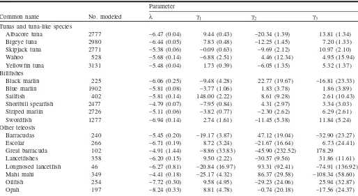
Common name No. modeled λ γ1 γ2 γ3
Tunas and tuna-like species
Albacore tuna 2777 –6.47 (0.04) 9.44 (0.43) –20.34 (1.39) 13.81 (1.34)
Bigeye tuna 2980 –6.44 (0.05) 7.83 (0.48) –12.25 (1.45) 7.20 (1.33)
Skipjack tuna 2771 –5.38 (0.06) –0.09 (0.63) –9.69 (2.12) 10.97 (2.10)
Wahoo 528 –5.68 (0.14) –6.88 (2.51) 4.46 (12.34) 4.95 (15.94)
Yellowfin tuna 3131 –5.48 (0.04) 1.73 (0.39) –6.05 (1.35) 5.32 (1.37)
Billfishes
Black marlin 225 –6.06 (0.25) –9.48 (4.28) 22.77 (19.67) –16.81 (23.33)
Blue marlin 1902 –5.81 (0.08) –3.77 (1.06) 1.83 (3.78) 1.86 (3.89)
Sailfish 402 –5.81 (0.14) 148.00 (2.22) 8.61 (9.28) 2.61 (10.43)
Shortbill spearfish 2477 –4.79 (0.07) –7.95 (0.84) 4.31 (2.97) 3.34 (3.03)
Striped marlin 2726 –5.11 (0.06) –3.82 (0.77) –2.30 (2.62) 6.29 (2.61)
Swordfish 1277 –6.94 (0.14) 2.74 (1.61) –11.45 (5.38) 11.84 (5.24)
Other teleosts
Barracudas 240 –5.45 (0.20) –19.17 (3.87) 47.12 (19.04) –32.90 (23.27)
Escolar 266 –6.71 (0.19) 8.72 (3.24) –21.67 (16.64) 6.73 (24.41)
Great barracuda 102 –4.91 (1.44) –8.86 (33.83) –45.90 (232.52) 178.29
Lancetfishes 358 –6.20 (0.15) 9.50 (2.22) –30.57 (9.56) 31.86 (11.61)
Longnosed lancetfish 46 –6.27 (0.81) –20.84 (16.97) 93.31 (92.41) –74.91 (136.92)
Mahi mahi 349 –4.41 (0.18) –25.17 (4.32) 86.37 (29.58) –108.34 (58.60)
Oilfish 254 –7.72 (0.30) 9.58 (4.95) –29.23 (24.06) 25.94 (32.87)
Opah 197 –8.24 (0.33) 8.81 (4.78) –0.74 (20.18) –17.56 (24.37)
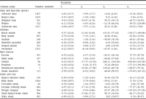
Parameter
Common name No. modeled λ γ1 γ2 γ3
Pomfrets 179 –6.95 (0.31) 6.69 (4.92) –29.87 (21.93) 38.71 (26.09)
Shortnosed lancetfish 53 –7.41 (0.45) –2.93 (6.33) 51.76 (27.49) –70.62 (35.01)
Sickle pomfret 20 –8.87 (1.08) 20.50 (17.01) –73.37 (79.15) 102.60 (106.75)
Snake mackerel 102 –6.34 (0.33) –11.78 (6.06) 63.10 (30.00) –72.36 (42.00)
Sharks and rays
Bigeye thresher shark 956 –8.08 (0.21) 7.88 (1.98) –12.95 (5.69) 8.52 (4.98)
Blue shark 3050 –5.43 (0.05) 0.35 (0.52) –0.77 (1.68) –0.16 (1.62)
Common thresher shark 30 –7.67 (1.52) –2.40 (27.45) 59.64 (149.25) –135.85 (247.22)
Crocodile shark 384 –7.79 (0.30) 7.17 (3.18) –18.88 (9.83) 16.39 (9.14)
Dusky shark 54 –4.55 (0.57) –19.05 (7.22) 47.48 (25.06) –35.91 (25.48)
Grey reef shark 25 –6.51 (0.56) 3.43 (16.68) –46.59 (130.00) 101.53 (283.53)
Long-finned mako shark 153 –6.00 (0.29) –6.66 (4.00) 9.83 (14.42) –1.46 (14.66)
Oceanic whitetip shark 1910 –4.92 (0.07) –9.85 (0.97) 11.61 (3.48) –2.09 (3.56)
Pelagic stingray 356 –5.85 (0.15) –9.97 (2.65) 28.78 (12.82) –24.50 (16.14)
Short-finned mako shark 665 –6.14 (0.18) –9.11 (2.33) 26.32 (8.22) –22.57 (8.45)
Silky shark 1019 –5.17 (0.08) –3.56 (1.00) –4.43 (3.76) 9.90 (4.02)
Silver–tip shark 29 –6.34 (0.66) 12.75 (15.51) –162.55 (105.60) 407.47 (211.62)
Tiger shark 34 –5.03 (0.69) –27.92 (10.81) 91.35 (43.29) –87.35 (49.00)
Whip stingray 19 –2.69 (0.86) –75.92 (15.42) 298.97 (64.83) –322.17 (76.22)
Table A1(concluded).
Parameter
Common name Number modeled λ γ1 γ2 γ3
Tunas and tuna-like species
Albacore tuna 1267 –4.92 (0.17) –3.99 (2.17) 14.44 (8.43) –13.26 (9.83)
Bigeye tuna 1819 –5.53 (0.07) –1.50 (1.00) 8.32 (4.10) –7.84 (4.76)
Skipjack tuna 241 –5.63 (0.26) –10.47 (4.74) 39.32 (24.12) –44.72 (34.83)
Wahoo 122 –6.12 (0.29) –3.83 (8.24) –12.18 (64.44) 59.35 (128.00)
Yellowfin tuna 1417 –5.00 (0.07) –7.97 (1.14) 25.43 (5.58) –25.02 (7.89)
Billfishes
Black marlin 98 –5.57 (0.24) –21.65 (8.46) 151.63 (77.45) –310.27 (189.09)
Blue marlin 593 –5.70 (0.10) –7.35 (1.91) 24.06 (9.64) –22.96 (13.05)
Sailfish 148 –6.19 (0.21) 1.58 (5.16) –39.99 (34.39) 69.81 (47.04)
Shortbill spearfish 269 –6.56 (0.29) –0.08 (4.34) 8.10 (18.86) –16.20 (23.66)
Striped marlin 743 –6.35 (0.16) 0.88 (2.37) 6.05 (10.39) –12.54 (13.72)
Swordfish 2332 –6.22 (0.07) 16.38 (0.95) –47.07 (3.54) 39.58 (3.87)
Other teleosts
Escolar 107 –6.55 (0.28) 6.57 (5.19) –28.51 (26.10) 37.79 (35.79)
Mahi mahi 157 –6.09 (0.23) 3.88 (5.65) –48.80 (37.60) 74.12 (51.85)
Oilfish 96 –6.25 (0.43) –17.73 (14.76) 268.21 (144.36) –854.80 (410.20)
Pomfrets 35 –6.58 (0.54) –5.46 (13.57) 75.28 (99.03) –177.15 (195.89)
Shortnosed lancetfish 7 –4.76 (1.18) –32.04 (17.98) 145.64 (69.78) –168.07 (79.16)
Snake mackerel 113 –5.99 (0.29) –6.92 (9.85) 48.80 (95.07) –133.89 (243.15)
Sharks and rays
Bigeye thresher shark 139 –6.58 (0.29) –1.20 (4.43) 10.49 (18.75) –16.13 (22.29)
Blue shark 2444 –5.00 (0.07) 5.79 (0.84) –19.62 (3.15) 17.38 (3.34)
Crocodile shark 84 –6.55 (0.40) 1.44 (5.97) –4.02 (24.39) 4.66 (27.48)
Oceanic whitetip shark 494 –4.97 (0.11) –17.14 (2.39) 66.41 (14.78) –77.27 (26.39)
Pelagic stingray 204 –6.00 (0.24) –5.54 (6.86) 43.57 (56.22) –119.38 (127.20)
Short-finned mako shark 388 –5.74 (0.20) –13.66 (3.31) 58.33 (16.64) –66.17 (24.42)
Silky shark 362 –4.99 (0.12) –3.90 (2.71) 3.82 (19.07) –5.10 (30.97)