Toeplitz Quantization and Asymptotic Expansions:
Geometric Construction
⋆Miroslav ENGLIˇS †‡ and Harald UPMEIER §
† Mathematics Institute, Silesian University at Opava, Na Rybn´ıˇcku 1, 74601 Opava, Czech Republic
‡ Mathematics Institute, ˇZitn´a 25, 11567 Prague 1, Czech Republic
E-mail: [email protected]
§ Fachbereich Mathematik, Universit¨at Marburg, D-35032 Marburg, Germany
E-mail: [email protected]
Received October 01, 2008, in final form February 14, 2009; Published online February 20, 2009
doi:10.3842/SIGMA.2009.021
Abstract. For a real symmetric domain GR/KR, with complexificationGC/KC, we
intro-duce the concept of “star-restriction” (a real analogue of the “star-products” for quantiza-tion of K¨ahler manifolds) and give a geometric construction of theGR-invariant differential
operators yielding its asymptotic expansion.
Key words: bounded symmetric domain; Toeplitz operator; star product; covariant quanti-zation
2000 Mathematics Subject Classification: 32M15; 46E22; 47B35; 53D55
1
Introduction
Geometric quantization of (complex) K¨ahler manifolds is of particular interest for symmetric
manifolds B=G/K (of compact or non-compact type). In this case the Hilbert state spaceH
carries an irreducible representation of G, whereas the various star products (Weyl calculus, Toeplitz–Berezin calculus) describe the (associative) product ofobservables (operators onH) as an asymptotic series of G-invariant bi-differential operators onB.
In this paper we introduce and study similar concepts forreal symmetric manifolds (of flat or non-compact type), emphasizing the interplay between the real symmetric space and its “hermitification” which is a complex hermitian space (of flat or non-compact type). In general, for a real-analytic manifoldBRof dimension n, a complexificationBC is a complex manifold of
(complex) dimension n, with BR embedded (real-analytically) as a totally real submanifold [1, 16,29]. IfBR=GR/KRis a symmetric space, for a real (reductive) Lie groupGR with maximal
compact subgroup KR, we write its hermitification as BC = GC/KC, where GC denotes the
(real, semi-simple) biholomorphic isometry group and KC is the maximal compact subgroup.
Thus, contrary to the usual notational conventions, GC is not the complexification of GR but
the real Lie group “in the complex setting”. For example, ifGR=SU(1,1) then GC is given by
SU(1,1)×SU(1,1) instead ofSL(2,C); similarly, for GR=SO(1,1) we have GC=SU(1,1). On the level of states, the interplay between a real symmetric space BR = GR/KR and
its hermitification BC = GC/KC corresponds to a “real-wave” realization of HC via a Segal–
Bargmann transformation [37], which is invariant under the subgroupGR ⊂GC. On the other
hand, the real analogue of the star-product is not so obvious. In this paper (and its companion paper [22]) we introduce such a concept, called “star-restriction” for real symmetric domains
⋆This paper is a contribution to the Special Issue on Deformation Quantization. The full collection is available
of non-compact type and study its asymptotic expansion as a series ofGR-invariant differential
operators. Whereas the paper [22] establishes existence and uniqueness of the asymptotic expan-sion, closely related to spectral theory and harmonic analysis (spherical functions), the current paper gives a “geometric construction” of the differential operators involved, based on a GR
-invariant retractionπ :BC→BR.
We emphasize that our∗-restriction operator is a GR-equivariant map
C∞(BC)→ C∞(BR)
instead of a map C∞(BR)⊗ C∞(BR) → C∞(BR) analogous to the usual ∗-products. Thus we
do not propose a quantization method for general real symmetric domains (which may not be symplectic nor even dimensional) but instead consider invariant operators which somewhat resemble boundary restriction operators such as Szeg¨o or Poisson kernel integrals. In caseBR is
the underlying real manifold of a complex hermitian domainB, then both concepts coincide and indeed yield the well-known covariant quantization methods applied to the K¨ahler manifold B. In order to illustrate the two concepts, consider the simplest non-flat case of the open unit diskB⊂Cand its real formBR= (−1,1)⊂R. The complexificationBRCcoincides withB, and
we have a restriction operator ρ, mapping a smooth function f onB =BC
R to its restrictionρf
on BR. A star-restriction is a deformation of the operator ρ, obtained by adding smooth,
but non-holomorphic, differential operators on B as higher order terms. In the context of symmetric domains, these differential operators should be invariant under the subgroup GR of
the holomorphic automorphism group Gof B which leaves BRinvariant.
Now consider instead the (usual) complex situation. HereB is regarded as areal (symplectic) manifold, denoted by BR
, whose complexification BR
C is the product of B and its complex
conjugate B, with BR
embedded as the diagonal. Then a star-product, regarded as a bilinear operator acting on f ⊗g (with f, g smooth functions on B), is precisely a deformation of the usual product f ·g by (G-invariant) bi-differential operators on B or, equivalently, differential operators on BR
C = B×B. Since f ·g is nothing but the restriction of f ⊗g to the diagonal
BR
⊂ BR
C, we see that the concept of star-restriction yields in fact the star-product for the
special case where the complexified domain is of product type. The higher-dimensional case is analogous.
In order to state our main result concerning the asymptotic expansion (in the deformation parameter ν) of a ∗-restriction operator as above, we first note that for the basic Toeplitz– Berezin calculus (the only case considered in detail here) the ∗-restriction operator is trivial for anti-holomorphic functions so that we may concentrate on the holomorphic part, which is a GR-covariant map
ρν : O(BC)→ C∞(BR).
Using deep facts from representation theory (of the compact Lie groups KR and KC), we
con-struct a family of differential operators
ρm: O(B
C)→ C∞(BR)
indexed by integer partitions m1 ≥ · · · ≥ mr ≥ 0 (cf. Definition 3.1), and (in Theorem 3.1)
expressρν as an asymptotic series
ρν ∼ X
m
1 [ν]m ρ
m, (1.1)
Using the Fourier–Helgason transform onBR, it is conceivable (see [22] for the details) that
ρν can also be expressed as an oscillatory integral
ρνF(x)∼ Z
BC
F(z)aν(z, x)eνS(z,x)dz, (1.2)
where aν is a suitable power series in 1ν, and the “phase” S is a function onBC×BR invariant
under the diagonal action of GR. This is reminiscent of the WKB-quantization programme
of Karasev, Weinstein and Zakrzewski [35], studied extensively in the context of symplectic (i.e. not necessarily Hermitian, or even Riemannian) symmetric spaces by Bieliavsky, Pevzner, Gutt, and other authors, see e.g. [11, 10, 12, 13]. As has already been pointed out above, real symmetric domains need not be symplectic (in fact, they can even be of odd dimension), so neither of the two approaches contains the other, and the situations where they both apply include the original K¨ahler case of an Hermitian symmetric space. A thorough comparison of both methods is, however, beyond the scope of this paper. For the flat cases of BR =Rd and
BR = Cd, the expansions (1.2) were obtained quite explicitly, and for a whole one-parameter
class of calculi which includes the Toeplitz calculus, by Arazy and the second author [5]. In Section 4 the asymptotic series (1.1) are computed for the simplest cases of (real or complex) dimension 1. In general, finding explicit formulas may be quite difficult, but there is some hope that at least all symmetric domains of rank 1 (i.e., hyperbolic spaces in Rn,Cn,Hn and the Cayley plane) can be treated in a unified and explicit way.
2
Preliminaries
One of the most inspiring examples of deformation quantization is the Berezin quantization [7,8] using the Berezin transform and Toeplitz operators (originally called co- and contra-variant symbols, respectively). Although it has subsequently been generalized and extended to various classes of compact and noncompact K¨ahler manifolds [15, 19,28, 32], the theory is still richest in its original setting of complex symmetric spaces, or bounded symmetric domains, in Cd [9], due to the powerful machinery available from Lie groups and their representation theory on the one hand [26,34], and from the theory of Jordan triple systems on the other [30].
More specifically, let B = G/K be an irreducible bounded symmetric domain in Cd in the Harish-Chandra realization, with G the identity connected component of the group of all biholomorphic self-maps of B and K the stabilizer of the origin. For ν > p−1, p being the genus of B, let Hν2(B) denote the standard weighted Bergman space on B, i.e. the subspace of all holomorphic functions inL2(B, dµν), with
dµν(z) =cνK(z, z)1−ν/pdz,
wheredzstands for the Lebesgue measure,K(z, w) is the ordinary (unweighted) Bergman kernel of B, and cν is a normalizing constant to make dµν a probability measure. The space Hν2(B)
carries the unitary representationU(ν) of Ggiven by
Ug(ν)f(z) =f(g−1(z))·Jg−1(z)ν/p, g∈G, f ∈H2
ν(B),
where Jg denotes the complex Jacobian of the mappingg. (In general, ifν/pis not an integer,
then U(ν) is only a projective representation due to the ambiguity in the choice of the power
Jg−1(z)ν/p.)
By acovariant operator calculus, orcovariant quantization, onBone understands a mapping
A:f 7→ Af from functions onBinto operators onHν2(B) which isG-covariant in the sense that
In most cases, such calculi can be built by the recipe
Af = Z
B
f(ζ)Aζdµ0(ζ)
wheredµ0 is aG-invariant measure onB, and Aζ is a family of operators onHν2(B) labelled by
ζ ∈B such that
Ag(ζ)=Ug(ν)AζUg(ν)∗, ∀g∈G.
(One calls such a family acovariant operator fieldonB. One also usually normalizes the measure
dµ0 so thatA1 is the identity operator.) Note that in view of the transitivity of the action ofG
on B, any covariant operator field is uniquely determined by its value A0 at the originζ = 0.
The best known examples of such calculi are the Toeplitz calculus T and the Weyl calcu-lus W, corresponding to T0 = (·|1)1 (the projection onto the constants) and W0f(z) =f(−z)
(the reflection operator), respectively.
In addition to bounded symmetric domains, we will also consider the complex flat case of a Hermitian vector space B = Z ≈ Cd, with B = G/K for G the group of all orientation-preserving rigid motions of Z, and K = U(Z) ≈ Ud(C) the stabilizer of the origin in G;
the spaces Hν2(Z) will then be the Segal–Bargmann spaces of all entire functions which are square-integrable with respect to the Gaussian measure
dµν(z) = ν
π
d
e−νkzk2dz,
and U(ν) will be the usual Schr¨odinger representation. In this setting, the Weyl calculus W above is just the well-known Weyl calculus from the theory of pseudodifferential operators [25]. Given a covariant operator calculus A, the associated star product ∗ on functions on B is defined by
Af∗g =AfAg. (2.1)
It follows from the construction that the star-product is G-invariant in the sense that
(f◦φ)∗(g◦φ) = (f∗g)◦φ ∀φ∈G. (2.2)
While f∗g is a well-defined object for some calculi (e.g. for A =W, at least on Cd and rank one symmetric domains, see [5]), in most cases (e.g. forA=T, the Toeplitz calculus), it makes sense only for very special functions f,gand (2.1) is then usually understood as an equality of asymptotic expansions as the Wallach parameter ν tends to infinity. For instance, for A=T, it was shown in [14] that for anyf, g∈ C∞(B) with compact support,
kTfTg− TPN
j=0ν−jCj(f,g)k=O ν −N−1
as ν → ∞, for some bilinear differential operators Cj (not depending onf,g and ν). (The
as-sumption of compact support can be relaxed [18].) We can thus definef∗g as the formal power series
f ∗g:=
∞ X
j=0
ν−jCj(f, g).
and the definition (2.1), is not the traditional way of constructing theG-invariant Berezin quan-tization, however, for the case of bounded symmetric domains these two are equivalent [20].)
Viewing the Planck parameterν as fixed for the moment, the formula (2.2) means that one can view ∗ as a mapping from the tensor product
∗: C∞(B×B)∼=C∞(B)⊗ C∞(B)→ C∞(B), f⊗g→f ∗g,
which intertwines the G-action f 7→ f ◦ φ, φ ∈ G, on C∞(B) with the diagonal G-action
f⊗g7→(f◦φ)⊗(g◦φ) ofGonC∞(B×B). This observation can be used as a starting point for extending the whole quantization procedure also toreal bounded symmetric domainsBR⊂Rd,
as follows.
Suppose ZC is an irreducible hermitian Jordan triple [30, 34] endowed with a
(conjugate-linear) involution
z7→z#
which preserves the Jordan triple product and therefore the unit ballBCofZC, i.e. (BC)#=BC.
Define the real forms
ZR:={z∈ZC:z#=z},
BR:={z∈BC:z#=z}=Z∩BC.
For the groups GC:= Aut(BC), KC:= Aut(ZC) we have the subgroups
GR:={g∈GC:g(z#) =g(z)#},
KR:={k∈KC:kz#= (kz)#}=GR∩KC
acting onBRandZR, respectively. In this situationZRis an irreducible real Jordan triple,GRis
a reductive Lie group (it may have a nontrivial center), and
BR=GR/KR
is an irreducible real bounded symmetric domain. Up to a few exceptions, all non-hermitian Riemannian symmetric spaces of non-compact type arise in this way [30, Chapter 11].
Acovariant quantization (orcovariant extension) on the real bounded symmetric domainBR
is a map f 7→ Af fromC∞(BR) intoHν2(BC) such that Af◦g =Ug(ν)∗Af
for all g ∈ GR. The counterpart of the star product, associated to a covariant quantization A
on BR and a covariant quantization AC onBC, is the star restriction
ρ=ρν : C∞(BC)→ C∞(BR)
defined by
AρF =ACFI, (2.3)
where
I(z) =Iν(z) =K(ν)(z, z#)1/2
is the uniqueGR-invariant holomorphic function onBCsatisfying I(0) = 1. In addition, we will
involutive Hermitian vector space ZC ≈ Cd, with the ordinary complex conjugation as the
involution z7→z#; thusB=Z
R≈Rd.
In most cases, covariant extensions can again be constructed by the recipe
Af = Z
BR
f(ζ)Aζdµ0(ζ),
wheredµ0 is theGR-invariant measure in BR, and Aζ is a family of holomorphic functions (not
necessarily belonging to Hν2(BC)) labelled byζ ∈BR which is covariant in the sense that
Ag(ζ)=Ug(ν)Aζ, ∀g∈GR, ζ ∈BR.
As before, one usually normalizes dµ0 so that A1 = I. The prime example is now the real
Toeplitz calculus A=T corresponding to A0=1 (the function constant one) [36,31,17,6,3];
there is also a notion of real Weyl calculus, but it is more complicated [4].
Here is how the complex hermitian case of a bounded symmetric domainB ⊂Cd from the beginning of this section can be recovered within the more general real framework. Identify B
with the “diagonal” domain
BR:={(z, z) :z∈B} ⊂ZR:={(z, z) :z∈Z},
where the bar indicates that we consider the “conjugate” complex structure for the second component. The complexifications
BRC={(z, w) :z, w∈B}=B×B,
ZCR={(z, w) :z, w∈Z}=Z×Z
are endowed with the flip involution
(z, w)#:= (w, z)
having fixed pointsBR
andZR
, respectively. Similarly we can identify G,K with the groups
GR:={(g, g) :g∈G}, KR:={(k, k) :k∈K}
which act “diagonally” on BR
and ZR
, respectively, and whose complexifications
GC:={(g1, g2) :g1, g2 ∈G}=G×G,
KC:={(k1, k2) :k1, k2∈K}=K×K
act onBC andZC, withBC=GC/KC.
Since Hν2(B) is a reproducing kernel space (with reproducing kernel K(ν)(x, y) = h(x, y)−ν, where h(x, y) = [K(x, y)/cp]−1/p is the Jordan determinant polynomial), any bounded linear
operator on H2
ν(B) is automatically an integral operator: namely,
T f(z) =
Z
B
f(w)Te(z, w)dµν(w),
with
e
T(z, w) = (T∗K(ν)(·, z))(w) = (T K(ν)(
·, w)|K(ν)(·, z)).
anti-holomorphic in the second variable; that is, with holomorphic functions onBC. Upon this
identification, the covariant quantization rule f 7→ Af becomes simply a (densely defined)
operatorf 7→Aef from C∞(BR) into the Hilbert space
Hν2(BC)≈Hν2(B)⊗Hν2(B)
corresponding to the Hilbert–Schmidt operators, and the covariance condition means that Ae is equivariant under GR ≈ G, i.e. intertwines the G-action on the former with the diagonal
G-action on the latter:
e
Af◦g = Ug(ν)∗⊗Ug(ν)∗ eAf.
Similarly, upon takingAC
=A⊗A, and identifying pairsf,gof functions onBwith the function
F(x, y) = f(x)g(y) on BC, (2.3) reduces just to (2.1). Note, however, that the complexified
domain BC is now no longer irreducible, but of “product type”. We will henceforth refer to
this situation, i.e. of BR =B,BC =B×B with a bounded symmetric domainB ⊂Cd, as the
“complex” case.
To each covariant extension (or quantization)Awe can consider its adjointA∗ fromH2
ν(BC)
into functions on BR, defined with respect to the inner products inHν2(BC) and L2(BR, dµ0).
That is,
(A∗f|φ)L2 = (f|Aφ)ν, ∀φ∈L2(BR, dµ0), ∀f ∈Hν2(BC). (2.4)
One sometimes calls A∗ a covariant restriction; this should not be confused with the
star-restriction ρ, which is a map fromC∞(BC) into functions onBR.
One can also consider the associated link transform, which is the composition A∗A, a GR
-invariant operator on functions on BR. In particular, for the Toeplitz calculus A=T, the link
transform
T∗T =:Bν
is theBerezin transform, introduced for the ‘complex‘” case in Berezin’s original papers (cf. Sec-tion 4 below).
A crucial role in the analysis on complex bounded symmetric domains is played by the Peter– Weyl decomposition of holomorphic functions on B under the composition action f 7→f ◦kof the (compact) group K. Namely, the vector space P of all holomorphic polynomials on Cd decomposes under this action into non-equivalent irreducible components
P =X
m
Pm
labelled bypartitions (or signatures) m∈N+r, that is, by r-tuples of integersm1 ≥m2 ≥ · · · ≥
mr≥0, where r is the rank ofB. With respect to the Fock inner product
(p|q)F := Z
Cd
p(z)q(z)e−|z|2dz=p(∂)q∗(0), q∗(z) :=q(z#),
each Peter–Weyl spacePm possesses a reproducing kernelKm(z, w),z, w∈Z. It was shown by
Arazy and Ørsted [2] that the Berezin transform Bν admits the asymptotic expansion
Bν = X
m
Em
whereEmis theG-invariant differential operator onBdetermined (uniquely) by the requirement that
Emf(0) =Km(∂, ∂)f(0), ∀f ∈ C∞(B);
while (ν)m is the multi-Pochhammer symbol
(ν)m =
r Y
j=1
Γ(ν−a2(j−1) +mj)
Γ(ν−a2(j−1)) ,
abeing the so-calledcharacteristic multiplicity ofB. Analogously, it was shown in [18] that the star-product (2.1) arising from the Toeplitz calculusA=T admits an expansion
f ∗g=X
m
Am(f, g)
(ν)m , (2.5)
where Am are certain (rather complicated) G-invariant (cf. (2.2)) bi-differential operators. The main purpose of the present paper is an extension of the last formula to real symmetric domains. That is, to obtain a decomposition of the star restriction operator
ρν = X
m
ρm
[ν]m (2.6)
with some GR-invariant differential operators ρm:C∞(BC)→ C∞(BR) (independent ofν) and
generalized “Pochhammer symbols” [ν]m.
A prominent role in our analysis is played by holomorphic polynomials on ZC which are
invariant under the group KR. In the Peter–Weyl decomposition under KC mentioned above,
partitions n for which Pn contains a nonzero KR-invariant vector are called “even”, and are
in one-to-one correspondence with partitions m of length rR = rankBR; furthermore, for each
“even” Peter–Weyl space the subspace of KR-invariant vectors is one dimensional, consisting
only of multiples of a certain polynomial which (under an appropriate normalization) we denote by Em. For more details, including the description ofEm, bibliographic references, etc., as well
as for the various preliminaries and notation not introduced here, we refer to [36,22].
The construction of the decomposition (2.6) for general real symmetric domains is carried out in Section 3. In Section4 it is shown that the decomposition obtained indeed reduces to (2.5) for the “complex” case. The final Section 5 contains a few examples with more or less explicit formulas forρm and [ν]
m. For the reader’s convenience, we are also attaching a table of all real
bounded symmetric domains and their various parameters.
In some sense, our results can be perceived as a step towards building a version of Berezin’s quantization for real (as opposed to K¨ahler) manifolds as phase spaces.
3
Invariant retractions and Moyal restrictions
As a first step towards a geometric construction of asymptotic expansions for the Moyal type restriction, we obtain an integral representation for the Moyal restriction operator, defined in terms ofGR-invariant retractions
π : BC→BR.
Here BR is an irreducible real symmetric domain of rank r, in its bounded realization (real
Cartan domain) and BC is the open unit ball of the complexification ZC, which is a complex
We will assume that the preimageπ−1(0) of the origin 0∈BR has the form
π−1(0) =BC∩Y = ΛBR (3.1)
for some real vector subspaceY ⊂BCand real-linearKR-invariant map Λ :ZR→ZC. Our
con-struction in fact works even without these assumptions (cf. Remark3.1below), but all situations studied in this paper will be of the above form.
LethC:ZC×ZC→ Cdenote the Jordan triple determinant (cf. [30]) of ZC and define the Berezin kernel
Bν : BC→C
by
Bν(z) :=hC(z, z)ν/|hC(z, z♯)|ν, (3.2)
where z7→z♯ is the involution with real formBR. Note that hC(z, w)6= 0 for allz, w ∈BC.
Proposition 3.1. The Berezin kernelBν isGR-invariant, i.e.,
Bν(gz) =Bν(z) for all g∈GR and z∈BC.
Proof . Since GR⊂GC we have
hC(gz, gw)ν =jν(g, z) hC(z, w)νjν(g, w)
for all z, w∈BC, where
jν(g, z) = [det g′(z)]ν/p
and p is the (complex) genus ofBC. Forg∈GR we have
g(z)♯=g(z♯)
and
jν(g, z) =jν(g, z♯)
since these relations are anti-holomorphic in z∈BC and hold forz=z♯. It follows that
hC(gz, gz)ν |hC(gz,(gz)♯)|ν
= hC(gz, gz)
ν
hC(gz, g(z♯))ν/2hC(g(z♯), gz)ν/2
= jν(g, z) hC(z, z)
ν j ν(g, z)
jν/2(g, z) hC(z, z♯)ν/2 jν/2(g, z♯)jν/2(g, z♯) hC(z♯, z)ν/2 jν/2(g, z)
= hC(z, z)
ν
|hC(z, z♯)|ν
jν/2(g, z) jν/2(g, z)
jν/2(g, z♯) j
ν/2(g, z♯)
= hC(z, z)
ν
|hC(z, z♯)|ν
.
Another proof can be given by observing that, using the familiar transformation rule for hC,
hC(gz, gz) |hC(gz, gz#)|
=
hC(z, z)hC(a, a) |hC(z, a)|2
hC(z, z
#)h
C(a, a)
hC(z, a)hC(a, z#)
= hC(z, z)
|hC(z, z#)|
hhC(a, z) C(a, z#)
,
where g ∈ GC and a =g−1(0). If g ∈ GR, then gz# = (gz)#, while hC(a, z#) = hC(a#, z) =
The relationship between the Moyal restriction operator
ρν : C∞(BC)→ C∞(BR)
and the Berezin kernelBν is given by the following result.
Proposition 3.2. ForG∈ O(BC) and F ∈ C∞(BC) we have, if ν is large enough, Z
BR
dx hC(x, x)
ν−p
2 G(x)(ρ
νF)(x) = Z
BC
dz hC(z, z)−pBν(z)(G/Iν)(z)F(z),
where
Iν(z) =hC(z, z♯)−ν/2.
Proof . The Toeplitz restriction mapT∗
R satisfies
(TR∗G)(x) =hC(x, x)ν/2G(x) = (G/Iν)(x)
for all x∈BR [36,6]. Using the duality relation (2.4) and the definition (2.3) ofρν we obtain Z
BR
dx hC(x, x)
ν−p
2 G(x) (ρ
νF)(x) = Z
BR
dx hC(x, x)−p/2(G/Iν)(x)(ρνF)(x)
=
Z
BR
dx hC(x, x)−p/2(TR∗G)(x)(ρνF)(x) = (TR∗G|ρνF)BR = (G|TRρνF)ν
= (G|TC(F)Iν)ν = (G|F·Iν)ν = Z
BC
dz hC(z, z)ν−pG(z)F(z)Iν(z)
=
Z
BC
dz hC(z, z)ν−p(G/Iν)(z)F(z)|Iν(z)|2.
Since
hC(z, z)ν|Iν(z)|2=Bν(z)
the assertion follows.
Corollary 3.1. For G∈ O(BC) and F ∈ C∞(BC), we have ρν(G F) =G ρνF.
It follows from (3.1) thatY ⊂ZC is aKR-invariant subspace such that
ZC=ZR⊕Y
(direct sum of real vector spaces). For x ∈ BR, let γx ∈ GR be the “transvection” sending 0
tox, explicitly given by
γx(y) =x+B(x, x)1/2(y−x),
where B is the Bergman operator and
yx=B(y, x)−1(y−Qyx)
Lemma 3.1. The mappingΦ :BR×(Y ∩BC)→BC defined by
Φ(x, y) =γx(y) (x∈BR, y ∈Y ∩BC)
is a real-analytic isomorphism, whose derivative at (0, y) is given by
Φ′(0, y)(ξ, η) =ξ+η− {yξy}
for all ξ∈ZR=Tx(BR), η∈Y =Ty(Y ∩BC).
Proof . For z ∈ BC, set x := πz and y = γ−xz (= γx−1z). Then x ∈ BR while, by the GR
-invariance ofπ,
πy=γ−xπz=γ−xx= 0,
so y ∈ Y ∩BC. This proves that Φ is surjective. Similarly, if Φ(x, y) = Φ(x′, y′) for some
x, x′ ∈ BR and y, y′ ∈ Y ∩BC, then x = γx0 = γxπy = πΦ(x, y) = πΦ(x′, y′) = x′ and
y=γ−xΦ(x, y) =γ−x′Φ(x′, y′) =y′, showing that Φ is injective. It remains to prove the formula
for the derivative. For this, we will use some of the formulas collected in [30, Appendix A1–A3]. For the quasi-inverse
Ψ(x, y) =xy
we obtain, by definition,
Ψ(ξ, y) =B(ξ, y)−1(ξ−Qξy)
and hence
(∂1Ψ)(0, y)ξ=ξ.
Using thesymmetry formula [30, A3] we obtain
Ψ(x, η) =xη =x+Qx(ηx) =x+Qx B(η, x)−1(η−Qηx)
and hence
(∂2Ψ)(x,0)η=Qxη.
Now the addition formulas [30, A3] yield
(x+ξ)y =xy+B(x, y)−1(ξ(yx)) and hence
(∂1Ψ)(x, y)ξ =B(x, y)−1(∂1Ψ)(0, yx)ξ =B(x, y)−1ξ.
Similarly, we have
x(y+η)= (xy)η
and hence, with (JP28) from [30, A2],
(∂2Ψ)(x, y)η = (∂2Ψ)(xy,0)η=Qxyη=B(x, y)−1Qxη.
It follows that
Since B(x, x)1/2 is an even function ofx, its derivative at x= 0 vanishes and we obtain for
Φ(x, y) =γx(y) =x+B(x, x)1/2y−x=x+B(x, x)1/2Ψ(y,−x)
the derivatives
∂1Φ(0, y)ξ=ξ−∂2Ψ(y,0)ξ=ξ−Qyξ
and
∂2Φ(0, y)η=∂1Ψ(y,0)η =B(y,0)−1η=η.
Therefore
Φ′(0, y)(ξ, η) = (∂1Φ)(0, y)ξ+ (∂2Φ)(0, y)η=ξ+η−Qyξ.
Corollary 3.2. For all y∈Y ∩BC we havedet Φ′(0, y) = detZR(I−Qy).
DefinePν :C∞(BC)→ C∞(BR) by
(PνF)(x) :=hC(x, x)p/2 Z
Y∩BC
dy F(γxy)|det Φ′(x, y)| ·hC(γxy, γxy)−pBν(y)
=hC(x, x)p/2 Z
Y∩BC
dy F(γxy)|det Φ′(x, y)|hC(γxy, γxy)ν−p|hC(γxy,(γxy)♯)|−ν
for all F ∈ C∞(B
C) andx∈BR. Here Φ′(x, y) is the derivative of Φ at (x, y)∈BR×(Y ∩BC).
If f ∈ C∞(B
R), thenf ◦π ∈ C∞(BC) and
(f◦π)(γxy) =f(γxπ(y)) =f(γx0) =f(x).
It follows that
Pν((f◦π)F) =f·(PνF), (3.3)
i.e. Pν behaves like a “conditional” expectation.
Proposition 3.3. ForF ∈ C∞(BC) we have Z
BR
dx hC(x, x)−p/2(PνF)(x) = Z
BC
dz hC(z, z)−pBν(z)F(z).
Proof . The change of variablesz=γx(y) = Φ(x, y) yields in view of the invariance of Bν Z
BC
dz hC(z, z)−pBν(z)F(z) = Z
BR
dx
Z
Y∩BC
dy|det Φ′(x, y)|hC(γxy, γxy)−pBν(y)F(γxy)
=
Z
BR
dx hC(x, x)−p/2(PνF)(x).
Corollary 3.3. The operator Pν isGR-invariant, i.e., we have
Pν(F◦g) = (PνF)◦g
Proof . Letf ∈ C∞(BR) be arbitrary. Using (3.3) and theGR-invariance ofBν andπ, we obtain stationary phase but also the more refined “KR-invariant” Taylor expansion of F at 0∈Y. As
a first step we recall that
Y = ΛZR={Λx: x∈ZR},
for an R-linear (but not necessarily C-linear) isomorphism Λ : ZC → ZC which commutes
with KR. Forf ∈ C∞(BR) we have f◦Λ−1 ∈ C∞(Y ∩BC). Consider the distribution
f 7→ Pν f◦Λ−1
(0) (3.5)
on BR, which by construction isKR-invariant. For any partition m ∈ Nr+ let ERm be the KR
-invariant constant coefficient differential operator on ZR corresponding to the polynomial Em
introduced in Section2. Using multi-indicesκ ∈Nd we may write
Em(x) =X
R determines a complexified constant coefficient differential operator
where
Pα,βm =X
σ,τ
cmσ,τ Λσ,τα,β. (3.6)
Returning to the distribution (3.5) on BR, one has
Proposition 3.4. There exist unique constants[ν]m, form∈Nr+, such that for allF ∈ C∞(BC)
(PνF)(0)∼ X
m
1 [ν]mE
m
C(F◦Λ)(0) (3.7)
as an asymptotic expansion.
Proof . By the definition ofY, the real-linear operatory7→y#fromY intoZC is injective, and
thus bounded below. It follows that also the (GC-invariant) pseudohyperbolic distance
ρ(y, y#) :=kγy(y#)k, y∈BC,
is bounded below by a multiple ofky−y#kify∈Y. Since, by the familiar transformation rule for the Jordan determinant hC,
Bν(z)2=
h(z, z)νh(z#, z#)ν
|h(z, z#)|2ν =h(γzz
#, γ
zz#)ν
and h(w, w) ≤ 1 on the closure of BC, with equality if and only if w = 0, it follows that Bν
has a global maximum on Y aty = 0, which also dominates the boundary values of Bν in the
sense that Bν(yk) → 1, yk ∈ Y, implies that yk → 0. We may therefore apply the method of
stationary phase exactly as in Section 3 of [22] to conclude that for anyF ∈ C∞(BC), for which
the right-hand side exists for some ν > p−1, the integral
PνF(0) = Z
Y
F(y)|det Φ′(0, y)|Bν(y)hC(y, y)−p/2dy
=|det Λ|
Z
BR
F(Λx)|det Φ′(0,Λx)|Bν(Λx)hC(Λx,Λx)−p/2dx
has an asymptotic expansion asν →+∞
PνF(0)∼ν−d/2 X
k≥0
Sk(∂R)(F◦Λ)(0)ν−k
for some constant coefficient differential operators Sk(∂R), with Sk polynomials on ZR. Since Pν isKR-invariant, so must be theSk; thus they admit a decomposition
Sk= X
|m|≤k
qkmEm, qkm∈C,
into the “even” Peter–Weyl components Em. Interchanging the two summations and setting
1 [ν]m :=ν
−d/2X
k
qkmν−k,
Using the transvectionsγx ∈GR, forx∈BR, we define a GR-invariant differential operator
Proof . Since γx preserves holomorphy, (3.10) implies
Pm(GH)(x) =X
Definition 3.1. Form∈Nr+, the m-th Moyal component is the differential operator
Proposition 3.5. Let G, H ∈ O(BC). Then
Proof . Since G is holomorphic, we have ∂κ
CG(x) = ∂ κ
RG(x) for all κ ∈ Nd and x ∈ BR.
Applying Lemma 3.2toG/Iν we obtain Z
As a consequence of Proposition3.5 we obtain
Corollary 3.4. The differential operators ρm are GR-invariant, i.e.,
ρm(H◦g)(x) = (ρmH)(g(x))
The main result of this section yields the desired asymptotic expansion of the Moyal type restriction operator ρν in terms of the invariant differential operators ρm:
Theorem 3.1. ForH ∈ O(BC) we have an asymptotic expansion
Remark 3.1. Most – probably all – of the above extends also to the case of generalGR-invariant
smooth retractions π : BC → BR, i.e. when π−1(0) is not necessarily an intersection of BC
with some real subspace Y, or that the parameterization Λ : BR → π−1(0) is not necessarily
linear but only smooth. In fact, the application of the stationary phase method in the proof of Proposition3.4involves only the germs ofF andπ−1(0) (or, equivalently, Λ) at the origin. Thus
we may replace the variety π−1(0) by its tangent space at 0 ∈ π−1(0), and Λ : BR → π−1(0)
by its differential at the origin. We omit the details.
4
Asymptotic expansion: the complex case
In the complex case, where
BC=B×B ={(z, w) : z, w∈B},
BR={(z, z) : z∈B}
and B is an irreducible complex Hermitian bounded symmetric domain (of rank r), the Moyal type restriction operator
ρν : C∞(BC) =C∞(B)⊗ C∞(B)→ C∞(BR)
can be identified with the Moyal type (star-) product♯ν via the formula
ρν(f⊗g) =f ♯νg
for all f, g ∈ C∞(B). In this case an asymptotic expansion has been constructed in [18], and here we show that the general construction described in Section3 yields precisely the expansion of [18]. This is not completely obvious, since the construction in [18] is based on the complex structure of B whereas the general construction of Section3 uses the “real” structure ofBR.
The first step is to identify the Berezin kernelBν on BC, defined in (3.2), for the complex
case. We have
hC((z, w),(ζ, ω)) =h(z, ζ)h(ω, w)
forz, w, ζ, ω∈B and the involution is given by
(z, w)♯:= (w, z).
Therefore
Bν(z, w) =
hC((z, w),(z, w))ν |hC((z, w),(w, z))|ν
= h(z, z)
νh(w, w)ν
h(z, w)ν h(w, z)ν
coincides with the integral kernel for the G-invariantBerezin transform
Bν : C∞(B)→ C∞(B)
on B. This is clearly invariant under
GR={(g, g) : g∈G},
where G= Aut (B). The construction in [18] starts with the asymptotic expansion
(Bνf)(0) = Z
B
dz h(z, z)ν−pf(z) =X
m
1 (ν)m(E
m
of the ν-Berezin transform Bν associated with the usual Toeplitz–Berezin quantization of B.
Here, for any partition m∈Nr
+, the Pochhammer symbol
(ν)m := ΓΩ(ν+m) ΓΩ(ν)
is defined via the Koecher–Gindikin Γ-function, and the “sesqui-holomorphic” constant coeffi-cient differential operators Em
R are defined via the Fock space expansion
e(z|w)=X
m
Em(z, w)
for all z, w∈Z. In multi-index notation,
Em(z, w) =X
α,β
cm
α,βzαwβ, ERm= X
α,β
cm
α β∂α∂β (4.1)
for suitable constants cm
α β and multi-indices α, β∈Nd, such that|α| ≤ |m| ≥ |β|. Since
Em(z, w) =Em(w, z)
it follows that
cm
α β =cmβ α. (4.2)
Passing to the complexification ZC=Z×Z, with variables (z, w) for z, w ∈Z, we use pairs of
multi-indices and write∂Cαβ and∂γδC for the associated Wirtinger derivatives. Thus, for functions
on BC of the form
(f⊗g)(z, w) =f(z)g(w), (4.3)
we have
∂Cαβ∂ γδ
C(f ⊗g) = (∂α∂γf)⊗(∂β∂δg). (4.4)
Note that the first and second variable are treated differently, since holomorphic functions onBC
correspond to the case where f is holomorphic andg is anti-holomorphic. Let
Λ : BR→BC
denote the R-linear mapping
Λ(z, z) = (z,0)
which is clearly KR-invariant. Consider theGR-invariant retraction
π : BC→BR
defined by π(z, w) := (w, w). Then
π−1(0) ={(z,0) : z∈B}= ΛBR.
Lemma 4.1. ForF ∈ C∞(B
C) we have
Em
C(F◦Λ)(0) = X
α,β
cm
α β∂Cα0∂ β0
Proof . We may assume that F(z, w) =f(z)g(w) is of the form (4.3) . Since
((f⊗g)◦Λ)(z, z) = (f ⊗g)(z,0) =f(z)g(0)
it follows from (4.4) and (4.1) that
Em
C((f⊗g)◦Λ)(0) = (Emf)(0)g(0) = X
α,β
cm
α β(∂α∂βf)(0)g(0)
=X
α,β
cm
α β(∂αC0∂ β0
C (f⊗g))(0).
Comparing with the coefficientsPm
α,β introduced by (3.6) in the general case, it follows that
Pαm0,β0 =cmα β (4.5)
forα, β ∈Nd, whereas all other such coefficients vanish. This reflects the fact that Λ is trivial on the second component. For z∈B, let as beforeγz ∈Gbe the transvection mapping 0 to z.
Then we have for α∈Nd and f ∈ O(B)
∂α(f◦γz)(0) = X
ι≤α
για(z)(∂ιf)(z),
where για are smooth functions on B. As in [18] define a G-invariant operator
Em : C∞(B)
→ C∞(B) by putting
(Emf)(z) :=ERm(f ◦γz)(0).
Then we have for f, g∈ O(B)
(Em(f g))(z) =Em
R((f g)◦γz)(0) =ERm((f◦γz)g◦γz)(0)
=X
α,β
cmα β∂α∂β((f ◦γz)g◦γz)(0) = X
α,β
cmα β∂α(f ◦γz)(0)∂β(g◦γz)(0)
=X
α,β X
κ,ι
cm
α βγκα(z)(∂ κ
f)(z)γιβ(z)(∂ιg)(z). (4.6)
Following [18, Section 4] one defines (non-invariant) differential operatorsRm
κ, for any partition
m∈Nr+ and any multi-indexκ∈Nd with|κ| ≤ |m|, via the expansion
(Em(f g))(z) =X
κ
(∂κf)(z)(Rm
κg)(z),
where f ∈ O(B), g∈ C∞(B). Comparing with (4.6) it follows that
(Rmκg)(z) = X
α,β X
ι
cmα βγκα(z)γ β
ι (z)(∂ιg)(z)
whenever g is holomorphic. On the other hand, putting
we have for the “holomorphic” Wirtinger derivatives
We will now compute the (non-invariant) operators Pm
κ , introduced in (3.10), for the complex
case. Combining (4.5) and (4.7) it follows that the non-zero operators correspond to multi-index pairs (κ,0) forκ∈Nd and, in view of (4.2),
This passing to the complex conjugate (also in the proof of the following Proposition) could be avoided by working with the “anti-holomorphic” second variable instead.
TheG-invariant bi-differential operatorsAm on B, introduced in [18, Section 4], satisfy
Am(f, g)(z) =X
κ
h(z, z)p(−∂)κ(h−pf(Rm
κ g))(z)
for all f, g ∈ O(B), and are uniquely determined by this property since Am involves only
holomorphic derivatives in the first variable and anti-holomorphic derivatives in the second variable. By [18, Proposition 6],
Am(f, g) =Am(g, f)
Proof . Since the operators ρm are defined by taking suitable adjoints on BR, which requires
=
Z
B
dz h(z, z)−pφ(z)ψ(z)A
m(g, f)(z) =
Z
B
dz h(z, z)−pφ(z)ψ(z)Am(f, g)(z).
Sinceφ, ψ∈ O(B) are arbitrary, the assertion follows. Note that the formula (3.11) definingρm
uses the real derivatives ∂R, whereas in this section we are using rather the Wirtinger
deriva-tives∂ and∂ on B (corresponding to viewingBR=B as a domain inCd rather thanR2d); this
is reflected by the appearance of the Hermitian adjoint −∂κ0 (rather than−∂κ0) of∂κ0 on the
third line in the computation above.
5
Examples
We begin with the case of the Euclidean space where everything can be computed explicitly.
Example 5.1. Let BR = R, so that BC = C, and Λx := εx for some ε ∈ C\R, |ε| = 1.
The corresponding retraction π is just the oblique R-linear projection associated to the direct sum decomposition
C=R⊕εR;
the mapping φ is just Φ(x, y) = x+y, and det Φ′ = 1. The role of the Jordan determinant
polynomial hC(x, y) is played by the function
e−xy, x, y∈C, (5.1)
and the “genus”p= 0 while “rank”r= 1. The partitions are just nonnegative integersm= (m), and the polynomialsEm are simply
Em(x) = x2m
(2m)!.
Thus Em
C = (∂+∂)2m/(2m)!, and
Pα,βm =
εα−β
α!β! ifα+β = 2m, 0 otherwise.
(5.2)
The “transvections” γx are just the ordinary translations γxy = x+y, which implies that the
functions γαι equal constant one if α = ι, and vanish otherwise. Feeding all this information into (3.10) and (3.11), we get
Pm
κ =
ε2m−2κ
(2m−κ)!κ! ∂
2m−κ
and, for H∈ O(C),
ρmH= 1
(2m)!
2m X
κ=0
2m
κ
ε2m−2κ(−1)κ∂Rκ(∂2m− κ
H) = (ε−ε)
2m
(2m)! ∂
2mH.
We next compute the “Pochhammer” symbols [ν]m, using the formula (3.4). By (5.1),
PνF(0) = Z
εR
F(y)e
−ν|y|2 |e−y2
|ν dy= Z
R
Denoting for brevity 1−Reε2 = −12(ε−ε)2 =: c > 0 and making the change of variable
We may assume that F is holomorphic; replacing then F by its Taylor expansion, integrating term by term (which is easily justified), and using the fact that RRx2je−x
where the last equality used the doubling formula for the Gamma function.
This corresponds to the unnormalized Lebesgue measure onC; it is usual to make a normal-ization so thatρν1=1, i.e. [ν](0)= 1. If this is done then (5.3) gets divided by the same thing
is independent of it, as it should.
A similar analysis can be done forBR=Rd,d >1; cf. the next example.
Example 5.2. BR = Cd ∼=R2d, so that BC =Cd×Cd, where as always we identify BR with {(z, z) :z∈Cd} ⊂BC. For Λ, we let
Λz= (z, az) (5.4)
with some fixed a∈C,a6= 1. The retractionπ is the oblique real-linear projection associated to the direct sum decomposition
with the usual multi-index notation. Recalling that the numbers Pm
it follows that
(Here we are again using the “double” Wirtinger derivatives∂Cαβ etc. as in Section4.) As in the
preceding example, the role of the “Jordan determinant” hC is played by the function
hC((z, w),(z1, w1)) =e−(z|z1)−(w1|w) (5.7)
cated at the end of the proof of Proposition4.1.) Thus, symbolically,
ρm= (−1)m
provided dz is normalized so that [ν]0= 1. Thus (under this normalization)
Note that, again,
Example 5.3. As a first “non-flat” situation, consider the unit interval BR = (−1,+1) with
complexification BC = D, the unit disc in C; and we take the same Λ as in Example 5.1,
This time explicit formulas are hard to come by, since the expressions για(x) are quite compli-cated. One has, of course, ρ(0)H =H, while
we arrive at the double series
The double sum on the right-hand side is the value at x=ε,y=εof the Horn hypergeometric function of two variables [23,§5.7.1]
F1 m+12,ν−21,ν−21, m+ν−12, x, y
and in general cannot be evaluated in closed form. For particular values ofε, there may be some simplifications; for instance, forε=ithe integral (5.8) becomes
1 [ν]m =
Z 1
0
tm−12(1−t)ν−2(1 +t)1−νdt
= Γ(m+
1
2)Γ(ν−1)
Γ(m+ν−12) 2F1 m+
1
2, ν−1;m+ν− 12;−1
,
where 2F1 is the ordinary Gauss hypergeometric function.
We remark that expressions involving values of2F1 at−1 occur as eigenvalues of the Berezin
(or “link”) transform corresponding to the Weyl calculus on rank 1 real symmetric spaces, cf. [5, Theorem 4.1]. (Also, Horn’s hypergeometric functions of another kind – namely, Φ2 in
the notation of [23] – appear in the formula for the harmonic Segal–Bargmann kernel on Cd, see [21]; it is however unclear if there is any deeper relationship.)
Example 5.4. In this final example we considerBR=D, embedded inBC=D×Din the usual
way as {(z, z) :z∈D}. For Λ we take the same map Λz= (z, az) as in Example 5.2, with some fixed a∈ C,a 6= 1. The corresponding retraction π : BC → BR assigns to (z, w) ∈D×D the (unique) point x∈D such that γxw=aγxz. (The existence of such x follows by the following argument. For any z, w, u, v∈D, the existence of g∈Gsuch that gz=u,gw=v is equivalent to the equality
ρ(z, w) =ρ(u, v) (5.9)
of the pseudohyperbolic distances ρ(u, v) := |1u−−uvv|. On the other hand, if u runs through the interval [0,min{1,|1a|}) and v =au, then ρ(u, v) runs from 0 to 1; thus (5.9) holds for some u. With gas above, take x=−g−1(0).)
The constants Pm
αβ,γδ are then still given by the formula (5.6) from Example 5.2, while the
corresponding functions γιηαβ are easily seen to be given byγιηαβ(z, w) =για(z)γηβ(w), where για
are the one-variable functions for the disc from the preceding example. By (3.11) we thus get forH(z, w) =f(z)g(w), f, g∈ O(D), andm= (m),
ρmH(z, z) = (1−zw)2X
κ,λ
(−∂w)κ(−∂z)λ
(1−zw)−2 X
α,β,γ,δ,ι,η
Pm
αβ,γδ
για(z)γηβ(w)γκγ(w)γδλ(z)∂ιf(z)∂ηg(w)
w=z.
Here again (−∂w)κ(−∂z)λ occurs rather than (−∂w)λ(−∂z)κ, and likewise γκγ(w)γλδ(z) rather
thanγκγ(z)γλδ(w), for the same reasons as in Example5.2and in the proof of Proposition 4.1.
For low values ofm, one computes thatρ(0)(f g) =f g(of course), while
ρ(1)(f g)(z) =−|1−a|2 1− |z|22f′(z)g′(z)
is the G-invariant operator from O(D×D) intoC∞(D) uniquely determined by
Computer-aided calculations give
ρ(2)(f g)(0) =−|1−a|
2
2
h
4(1 +|a|2)f′(0)g′(0)− |1−a|2f′′(0)g′′(0)i
and
ρ(3)(f g)(0) =−|1−a|
2
6
h
36(1 +|a|2+|a|4)f′(0)g′(0)−18|1−a|2(1 +|a|2)f′′(0)g′′(0)
+|1−a|4f′′′(0)g′′′(0)i.
To compute [ν]m, we note as in Example5.2 that for the function F ∈ C∞(D×D) given by
F(z, w) =zαzβwγwδ, where α+γ =β+δ=ρ,
one has by (3.7)
PνF(0) =aγaδ ρ!
[ν]ρ
.
On the other hand, since now det Φ′(0,Λy) = |1 −a|2(1− |a|2|y|4) by Lemma 3.1, we have from (3.4)
PνF(0) =aγaδ|1−a|2 Z
D
zρzρ 1− |a|2|z|4(1− |z|
2)ν(1− |az|2)ν |1−a|z|2|2ν
dz
(1− |z|2)2(1− |az|2)2.
Passing to polar coordinates, we thus obtain (writing m instead ofρ),
m!
[ν]m =|1−a|
2
Z 1
0
tm (1− |a|
2t2)
(1−t)2(1− |a|2t)2
(1−t)ν(1− |a|2t)ν
|1−at|2ν dt. (5.10)
Using series expansions, the integral can again be expressed in terms of Horn-type two-variable hypergeometric functions, and simplifies for some special values of a. In particular, for a = 0 the right-hand side of (5.10) is just
Z 1
0
tm(1−t)ν−2dt= m!Γ(ν+ 1) Γ(ν+m) ,
so that
1 [ν]m =
Γ(ν−1) Γ(ν+m),
or, upon renormalizing so that [ν]0= 1,
[ν]m = Γ(ν+m)
Γ(ν) = (ν)m,
in agreement with the result
ρν(f g) = X
m
Am(f, g) (ν)m
from [18] reviewed in Section 4. Similarly, fora=−1, (5.10) becomes
1 [ν]m =
4Γ(2ν−2)
or, upon renormalizing dz so that [ν]0 = 1,
1 [ν]m =
2 (2ν−1)m2
F1(2ν−1, m+ 1;m+ 2ν−1;−1).
Crude estimates also show that
[ν]m ∼ |1−a|2mνm
1−2(1 +|a|
2)
|1−a|2ν +O
1
ν2
asν →+∞, which can be used to check at least for the first few terms that, again,
ρν = X
m
ρm
[ν]m
is indeed independent of a, although both ρm and [ν]
m are not. Note that the retraction π in
this case (a=−1) is simply
π(z, w) =mz,w,
the geodesic mid-point betweenz and w.
A
Table of parameters of real bounded symmetric domains
The table on the next page lists the groupsGR,KR, the root type Σ, the rankrR, characteristic
multiplicities aR, bR, cR and the dimension d of real bounded symmetric domains BR, as well
as the analogous parameters rC, aC, bC of the complex domains BC and the labellings of BC
andBRfollowing the notation in [30, Chapter 11]. The table was mostly compiled using [37,26, 24] and [30]. The low-dimensional isomorphisms between the various types, and the resulting restrictions on subscripts needed in order to make the table entries non-redundant, can be found e.g. in the cited chapter in Loos [30]. As a matter of notation, we use Gn(K) and Up,q(K) for
the identity component of the general linear (resp. pseudo-unitary) group over K = R,C,H (= quaternions). Sp2r(K) is the 2r×2r-symplectic group over K=R,C, whereas On(H) is the
quaternion analogue ofOn(C) (usually denoted bySO∗(2n)).
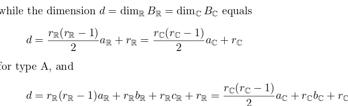
The genus ofBC is given in terms of the domain parameters by
p= (rC−1)aC+bC+ 2,
while the dimension d= dimRBR= dimCBCequals
d= rR(rR−1)
2 aR+rR=
rC(rC−1)
2 aC+rC for type A, and
d=rR(rR−1)aR+rRbR+rRcR+rR=
rC(rC−1)
2 aC+rCbC+rC
for all other types. Domains of type D2 turn out to have, in some sense, two multiplicities a
instead of one.
Note that the unit interval corresponds toIR
1,1, the unit ball ofRm,m >1, toI
R
1,m, the unit
ball of Cm to I1,m, the unit ball of the algebra of quaternionsH toI2H,2m, the unit ball ofHm,
m > 1, to IH
2,2m, and the unit ball of the Cayley plane O2 to V O
. In the “complex” cases, the root type does not quite make sense (“BC×BC”) and nor do the parameters aC, bC, rC,
M
.
E
n
gl
iˇs
an
d
H.
Up
m
ei
er
BR GR/KR Σ rR aR bR cR d rC aC bC BC
IR
r,r+b Ur,r+b(R)/Ur(R)×Ur+b(R) Dr/Br r 1 b 0 r(r+b) r 2 b Ir,r+b
Ir,r+b Ur,r+b(C)/Ur(C)×Ur+b(C) r 2 2b 1 2r(r+b) (product case)
IH
2r,2r+2b Ur,r+b(H)/Ur(H)×Ur+b(H) Cr/BCr r 4 4b 3 4r(r+b) 2r 2 2b I2r,2r+2b
VO0 U
2,2(H)/U2(H)×U2(H) B2 2 3 4 0 16 2 6 4 V
IIIR
r Gr(R)/Ur(R) Ar r 1 − − 12r(r+ 1) r 1 0 IIIr
IC
r,r Gr(C)/Ur(C) Ar r 2 − − r2 r 2 0 Ir,r
IIH
2r Gr(H)/Ur(H) Ar r 4 − − r(2r−1) r 4 0 II2r
V IO0 G
4(H)/U4(H) D3 3 4 0 0 27 3 8 0 V I
IIIr Sp2r(R)/Ur(C) r 1 0 1 r(r+ 1) (product case)
IIIH
2r Sp2r(C)/Ur(H) Cr r 2 0 2 r(2r+ 1) 2r 1 0 III2r
II2Rr+ε O2r+ε(C)/U2r+ε(R) Dr/Br r 2 2ε 0 r(2(r+ε)−1) r 4 2 II2r+ε
II2r+ε O2r+ε(H)/U2r+ε(C) r 4 4ε 1 2r(2(r+ε)−1) (product case)
IVpR+,qq SOp,1×SO1,q/SOp,0×SO0,q D2/A2 2 n/a 0 0 p+q 2 p+q−2 0 IVp+q
IVn SOn,2/SOn,0×SO0,2 2 n−2 0 1 2n (product case)
V E6(−14)/Spin(10)×SO(2) 2 6 8 1 32 (product case)
IVnR,0 SOn,1/SOn,0 C1 1 − 0 n−1 n 2 n−2 0 IVn
VO
F4(−20)/SO(9) BC1 1 − 8 7 16 2 6 4 V
V I E7(−25)/E6×SO(2) 3 8 0 1 54 (product case)
V IO
Acknowledgements
Research supported by the German-Israeli Foundation (GIF), I-696-17.6/2001; the Academy of Sciences of the Czech Republic institutional research plan no. AV0Z10190503; and GA ˇCR grant no. 201/06/0128.
References
[1] Akhiezer D.N., Gindikin S.G., On Stein extensions of real symmetric spaces,Math. Ann.286(1990), 1–12.
[2] Arazy J., Ørsted B., Asymptotic expansions of Berezin transforms,Indiana Univ. Math. J.49(2000), 7–30.
[3] Arazy J., Upmeier H., Covariant symbolic calculi on real symmetric domains, in Singular Integral Operators, Factorization and Applications,Oper. Theory Adv. Appl., Vol. 142, Birkh¨auser, Basel, 2003, 1–27.
[4] Arazy J., Upmeier H., Weyl calculus for complex and real symmetric domains,Atti Accad. Naz. Lincei Cl. Sci. Fis. Mat. Natur. Rend. Lincei (9) Mat. Appl.13(2002), 165–181.
[5] Arazy J., Upmeier H., A one-parameter calculus for symmetric domains,Math. Nachr.280(2007), 939–961.
[6] Arazy J., Upmeier H., Invariant symbolic calculi and eigenvalues of invariant operators on symmetric do-mains, in Function Spaces, Interpolation Theory, and Related Topics (Lund, 2000), Editors A. Kufner, M. Cwikel, M. Engliˇs, L.-E. Persson and G. Sparr, Walter de Gruyter, Berlin, 2002, 151–211.
[7] Berezin F.A., General concept of quantization,Comm. Math. Phys.40(1975), 153–174.
[8] Berezin F.A., Quantization,Math. USSR Izvestiya8(1974), 1109–1163.
[9] Berezin F.A., Quantization in complex symmetric spaces,Math. USSR Izvestiya9(1975), 341–379.
[10] Bieliavsky P., Strict quantization of solvable symmetric spaces, J. Symplectic Geom. 1 (2002), 269–320, math.QA/0010004.
[11] Bieliavsky P., Cahen M., Gutt S., Symmetric symplectic manifolds and deformation quantization, in Modern Group Theoretical Methods in Physics (Paris, 1995), Math. Phys. Stud., Vol. 18, Kluwer Acad. Publ., Dordrecht, 1995, 63–73.
[12] Bieliavsky P., Pevzner M., Symmetric spaces and star representations. II. Causal symmetric spaces,J. Geom. Phys.41(2002), 224–234,math.QA/0105060.
[13] Bieliavsky P., Detournay S., Spindel P., The deformation quantizations of the hyperbolic plane,
arXiv:0806.4741.
[14] Borthwick D., Lesniewski A., Upmeier H., Non-perturbative deformation quantization on Cartan domains, J. Funct. Anal.113(1993), 153–176.
[15] Bordemann M., Meinrenken E., Schlichenmaier M., Toeplitz quantization of K¨ahler manifolds and gl(n), n→ ∞limits,Comm. Math. Phys.165(1994), 281–296,hep-th/9309134.
[16] Burns D., Halverscheid S., Hind R., The geometry of Grauert tubes and complexification of symmetric spaces,Duke Math. J.118(2003), 465–491,math.CV/0109186.
[17] van Dijk G., Pevzner M., Berezin kernels and tube domains,J. Funct. Anal.181(2001), 189–208.
[18] Engliˇs M., Berezin–Toeplitz quantization on the Schwartz space of bounded symmetric domains, J. Lie Theory15(2005), 27–50.
[19] Engliˇs M., Weighted Bergman kernels and quantization,Comm. Math. Phys.227(2002), 211–241.
[20] Engliˇs M., Berezin–Toeplitz quantization and invariant symbolic calculi,Lett. Math. Phys.65(2003), 59–74.
[21] Engliˇs M., Berezin transform on the harmonic Fock space, in preparation.
[22] Engliˇs M., Upmeier H., Toeplitz quantization and asymptotic expansions for real bounded symmetric do-mains, Preprint, 2008,http://www.math.cas.cz/∼englis/70.pdf.
[23] Erd´elyi A. et al., Higher transcendental functions, Vol. I, McGraw–Hill, New York, 1953.
[24] Faraut J., Kor´anyi A., Analysis on symmetric cones, The Clarendon Press, Oxford University Press, New York, 1994.
[25] Folland G.B., Harmonic analysis in phase space,Annals of Mathematics Studies, Vol. 122, Princeton Uni-versity Press, Princeton, NJ, 1989.
[27] Hua L.K., Harmonic analysis of functions of several complex variables in the classical domains, American Mathematical Society, Providence, R.I., 1963.
[28] Karabegov A.V., Schlichenmaier M., Identification of Berezin–Toeplitz deformation quantization,J. Reine Angew. Math.540(2001), 49–76,math.QA/0006063.
[29] Lassalle M., S´eries de Laurent des fonctions holomorphes dans la complexification d’un espace sym´etrique compact,Ann. Sci. ´Ecole Norm. Sup. (4)11(1978), 167–210.
[30] Loos O., Bounded symmetric domains and Jordan pairs, University of California, Irvine, 1977.
[31] Neretin Yu.A., Plancherel formula for Berezin deformation ofL2on Riemannian symmetric space,J. Funct. Anal.189(2002), 336–408,math.RT/9911020.
[32] Reshetikhin N., Takhtajan L., Deformation quantization of K¨ahler manifolds, L.D. Faddeev’s Seminar on Mathematical Physics,Amer. Math. Soc. Transl. Ser. 2, Vol. 201, Amer. Math. Soc., Providence, RI, 2000, 257–276,math.QA/9907171.
[33] Schlichenmaier M., Deformation quantization of compact K¨ahler manifolds by Berezin–Toeplitz quanti-zation, Conference Mosh´e Flato, Vol. II (Dijon, 1999), Math. Phys. Stud., Vol. 22, Kluwer Acad. Publ., Dordrecht, 2000, 289–306,math.QA/9910137.
[34] Upmeier H., Toeplitz operators and index theory in several complex variables,Operator Theory: Advances and Applications, Vol. 81, Birkh¨auser Verlag, Basel, 1996.
[35] Weinstein A., Traces and triangles in symmetric symplectic spaces, in Symplectic Geometry and Quantiza-tion (Sanda and Yokohama, 1993),Contemp. Math.179(1994), 261–270.
[36] Zhang G., Berezin transform on real bounded symmetric domains, Trans. Amer. Math. Soc.353(2001),
3769–3787.