www.elsevier.com/locate/dsw
Improved dynamic programs for some batching problems
involving the maximum lateness criterion
A.P.M. Wagelmans
a;∗, A.E. Gerodimos
baEconometric Institute, Erasmus University Rotterdam, P.O. Box 1738, 3000 DR Rotterdam, Netherlands
bCentre for Quantitative Finance, Imperial College, Exhibition Road, London SW7 2BX, UK
Received 1 May 1999; received in revised form 1 November 1999
Abstract
We study four scheduling problems involving the maximum lateness criterion and an element of batching. For all the problems that we examine, algorithms appear in the literature that consist of a sorting step to determine an optimal job sequence, followed by a dynamic programming step that determines the optimal batches. In each case, the dynamic program is based on a backward recursion of which a straightforward implementation requires O(n2) time, where
nis the number of jobs. We present improved implementations of these dynamic programs that are based on monotonicity properties of the objective expressed as a function of the total processing time of the rst batch. These properties and the use of ecient data structures enable optimal solutions to be found for each of the four problems in O(nlogn) time; in two cases, the batching step is actually performed in linear time and the overall complexity is determined by the sorting step. c 2000 Elsevier Science B.V. All rights reserved.
Keywords:Batching; Scheduling; Dynamic programming; Computational complexity; Lateness
1. Introduction
The early 1990s saw the emergence of powerful techniques that reduced the time requirement of dynamic programming algorithms for the classic economic lot sizing (ELS) problem [8,14,1]. Subsequently, it was realized that certain scheduling problems involving the sum of completion times objective and an element of batching exhibited structural properties that made them amenable to more ecient dynamic programming solutions. In some cases [7,3], the improved schemes were problem-specic; in other cases [6,10], the dynamic programming recursion could be written in a form that allowed the application of the geometric techniques
of Van Hoesel et al. [13], which are a generalization of the technique used in [14]. The typical complexity improvement was from O(n2) to O(nlogn), where n is the number of jobs. A question that arises naturally
∗Corresponding author. Fax: +31-10-408-9162.
E-mail address:[email protected] (A.P.M. Wagelmans).
is whether similar improvements can be achieved in solving the maximum lateness counterparts of these batching problems since, in a standard implementation, the respective dynamic programs have also quadratic time requirements. This paper provides an armative answer to this question. We study four such batching problems and provide implementations of dynamic programming with a time requirement that is either linear or O(nlogn). Since the batching problems are solved after an initial sorting step, our results imply O(nlogn) algorithms for the four maximum lateness problems.
The remainder of this paper is organized as follows. In Section 2 we sketch our approach with particular focus on a subproblem that we encounter frequently when solving the four batching problems. Subsequently, we list the problems in order of relative complexity, both in terms of the improved running time and the diculty of obtaining this improvement. Specically, Section 3 deals with the problem of batching jobs of a single type under batch availability. A problem in which jobs are processed by a batching machine is the subject of Section 4. In Section 5 we give an improved algorithm for batching customized two-operation jobs on a single machine under batch availability and we indicate how a similar approach can be adopted in the case of item availability.
2. Preliminaries
In general, solving scheduling problems with a batching element involves taking the appropriate batching and sequencing decisions. For the problems that we examine in this paper, these two aspects can be decoupled. In fact, for three of our problems there is an optimal schedule in which jobs complete according to the earliest due date (EDD) rule, whereas for the problem studied in Section 4 the shortest processing time (SPT) rule is optimal. In any case, the sorting step imposes a lower bound of O(nlogn) on the overall complexity of any algorithm. For two of the problems examined here, improving the eciency of the dynamic programming step results in the sorting step being the overall bottleneck.
Although it is dicult to provide a description of a procedure that would be general enough to be applied to all the problems tackled in this paper, we now sketch some common elements of our approach; the implementation details and some special data structures deployed are covered in the subsequent sections.
Our starting point is always a backward recursion dynamic program with batch insertion [11]: for a pre-determined job sequence, the optimal schedule is built by inserting entire batches of jobs (or operations) at the start of previously obtained schedules. The recursions are of the general form:
Gk= min
k¡l6n+1{max{Pk; l+Gl; Lk; l}}; (1)
whereGk is the minimum lateness of schedules including jobsk; k+ 1; : : : ; n, whereas Pk; l andLk; l denote the
total processing time and overall lateness of the inserted batch, which consists of the jobs k; k+ 1; : : : ; l−1. In other words,lis the index of the rst job in the second batch. For a given choice ofl, the overall lateness of the schedule either occurs in the rst batch, in which case it is equal to Lk; l, or it occurs in the part of
the schedule starting with job l. The minimum lateness in the latter part of the schedule is simply the value
Gl corrected for the fact that job l starts at time Pk; l instead of time 0. This explains the termPk; l+Gl in
(1). The overall lateness of the schedule is given by the maximum of the lateness in the rst batch and the lateness in the remainder of the schedule. The minimum operation in (1) corresponds to the fact that the best possible choice for the start of the second batch is made.
The rst step in our approach is to observe that the index set {k+ 1; : : : ; n+ 1} can be partitioned into two mutually exclusive index sets Ik1 and Ik2 so that the rst set contains exactly those indices l for which
Pk; l+Gl¿Lk; l and the second set contains the remaining indices. In view of that, (1) can be re-written as
Gk= min
(
min
l∈I1
k
{Pk; l+Gl};min l∈I2
k
Lk; l
)
For reasons that will become clearer in the subsequent sections, the solution to the second minimization problem in (2) is obtained by retrieving the minimal index l∗
from I2
k. This leaves us with the following
tasks:
(a) maintain=update the index sets I1
k and Ik2 eciently;
(b) solve the rst minimization problem and, where applicable, a second optimization problem that arises when calculating Lk; l∗.
With respect to the rst task, observe that Ik1 and Ik2 are not necessarily contiguous. In fact, as we show in the subsequent sections, the satisfaction of this additional condition by some problems leads to linear-time implementations; where this is not the case, updating these index sets is “costly” and the complexity of the dynamic program becomes O(nlogn).
As for the second task, both the rst minimization problem and the non-trivial variants of the second optimization problem possess a key property that enables a solution to be found in time which is overall linear. Specically, the idea is to transform all such problems into a problem of the following type:
Problem P. Determine the minima mk, k= 1;2; : : : ; n;dened as
mk= min k¡l6uk
fl;
where uk∈ {k; k+ 1; : : : ; n} for all k= 1;2; : : : ; n (mk=∞ if uk=k) and the following conditions hold:
(a) uk6uk+1 for all k= 1;2; : : : ; n−1;
(b) un=n;
(c) uk is known once mk+1 is known; k= 1;2; : : : ; n−1;
(d) fk is known once mk is known; k= 1;2; : : : ; n:
Conditions (c) and (d) suggest that the values mk can only be calculated in order of decreasing index k. A
straightforward way to solve problem P requires O(n2) time. We show, however, that a linear time bound is
possible.
Consider, for an arbitrary k ∈ {1;2: : : ; n} with uk¿ k, the values fl; l=k+ 1; k+ 2; : : : ; uk. Let t(1); t(2); : : : ; t(r) be the unique subsequence of k+ 1; k+ 2; : : : ; uk which has the following properties:
1. t(1) =k+ 1;
2. t(i+ 1) is the smallest index in {t(i) + 1; t(i) + 2; : : : ; uk} such that ft(i+1)¡ ft(i), i= 1; : : : ; r−1.
Clearly, this subsequence has the propertiest(1)¡ t(2)¡· · ·¡ t(r) and ft(1)¿ ft(2)¿· · ·¿ ft(r). Moreover,
ft(r)=mk. Hence, given the subsequence, the desired minimum is immediately available.
We keep track of the subsequence by storing its elements in decreasing order in a doubly linked list (i.e,
fk+1 is the element at the top). This particular data structure has the property that elements can be deleted
from or added to the top or bottom of the list in constant time (see [2]).
To see why this data structure is convenient, rst observe the following: if for a given k¿2, a value
l∈ {k+ 1; k+ 2; : : : ; uk} is not selected in the subsequence, thenl will not be selected fork−1. This means that when for a certaink¿2 the elements t(1); t(2); : : : ; t(r) of the subsequence are given, then – onceuk−1 is
known – the corresponding subsequence for k−1 can be constructed as follows. Because uk−16uk, we rst
delete from the bottom of the list any element larger than uk−1. Now, suppose uk−1¿ k−1. Then, because
k will be added at the top of the list, we delete from the top all remaining elements t(i) for which fk6ft(i).
Finally, we add k at the top of the list. In case uk−1=k−1 the list is empty after the deletion operations
and no element is added.
the list elements are already ordered, each deletion requires indeed constant time. The number of deleted elements cannot be bounded nicely for each separate execution of the updating process. However, the overall number of deletions is not larger than n. The reason for this is simple: in the updating process, each of the elements 1;2; : : : ; n is added at most once to the list and therefore it can be deleted at most once.
To summarize the above discussion: we have shown that problem P can be solved in O(n) time. In the following sections, we will repeatedly have to calculate partial sums such as Pn
h=kph for all k = 1;2; : : : ; n. Note that this can be done in overall linear time in a preprocessing step. When needed, partial sums such as Pl−1
h=kph can subsequently be calculated in constant time as Pnh=kph−Pnh=lph.
3. Scheduling jobs of a single type under batch availability
The problem we are addressing in this section may be stated formally as follows. There are n jobs to be scheduled on a single machine. Each jobj(j= 1; : : : ; n) has a processing timepj and a due date dj by which
it should ideally complete. Jobs can be processed consecutively in batches. At the start of the schedule and prior to each batch, a set-up time s is incurred, which motivates the formation of longer batches so as to reduce the completion time of later jobs. However, batch availability applies, which means that all the jobs that belong to the same batch complete only when the last job in the batch completes. As a consequence, extending a batch by including additional jobs increases the completion time of the jobs previously in the batch.
The above problem setting is introduced in [12]. For the sum of completion times objective, an ecient algorithm is given by Coman et al. [7]: the batching step is performed in linear time to give an overall time requirement of O(nlogn). An extension of this algorithm for a slightly more general cost function is proposed by Albers and Brucker [3] (see also [5]). It is worth pointing out that the approach in [7,3], like ours, relies on the notion of a queue. However, in the problem examined here, the presence of a maximum operation within the dynamic programming recursion is an additional complication that does not arise in the sum of completion times variant. (This is also true for the problems addressed in later sections.)
It is shown in [15] that there is an optimal schedule in which jobs complete according to the earliest due date (EDD) rule. Thus, the jobs can be re-indexed according to this rule in O(nlogn) time and the problem reduces to one of batching that can be solved using a backward dynamic program with batch insertion. Let
Gk denote the minimum overall lateness of a schedule containing jobsk; k+ 1; : : : ; n when starting at time 0.
The initialization is Gn+1=−∞ and the recursion fork=n; n−1; : : : ;1 is
Gk= min k¡l6n+1
(
max
(
s+
l−1 X
h=k ph
!
+Gl; s+ l−1 X
h=k ph
!
−dk
))
; (3)
Here l denotes the rst job in the second batch of the schedule. Since this batch starts at times+Pl−1
h=kph,
the minimum overall lateness from this batch onward is given by the rst term between brackets, while the lateness of the rst batch is given by the other term (since job k has the smallest due date).
As pointed out in [15], a straightforward implementation of the above algorithm requires O(n2) time.
However, we now show that the dynamic programming part can be implemented in linear time. From (3) we have, for every l6n−1,
Gl+1= min
l+1¡i6n+1 (
max
(
s+
i−1 X
h=l+1
ph
!
+Gi; s+ i−1 X
h=l+1
ph
!
−dl+1 ))
which, because dl6dl+1, implies
Furthermore, it clearly holds that
Gl+16max{(s+pl) +Gl+1; (s+pl)−dl}: (5)
Combining (4) and (5) yields
Gl+16 min
From the above observations, it follows that for all indices l∈I1
k={k+ 1; : : : ; qk} the maximum in (3) is
given by the rst term, whereas for l∈I2
k ={qk+ 1; : : : ; n+ 1}, the maximum is given by the second term.
Now (3) can be rewritten as
Gk= min
Note that, for this problem, each ofI1
k andIk2is contiguous. Further, the second minimum is always attained
forl=qk+1: owing to the batch availability assumption and the EDD indexing of the jobs, the overall lateness
of a batch is always determined by the rst job in the batch. Consequently, the remaining task is to compute
s+
eciently. However, since this has to be done for every value of k, we actually need to solve an instance of problem P with uk=qk andfl=−Pnh=lph+Gl. As shown in Section 2, this problem can be solved in
O(n) time. Hence, it takes overall O(n) time to calculate the minima given by (6). Since the values Pn
h=lph, l= 1;2; : : : ; n, and, because of monotonicity, the values qk; k= 1;2; : : : ; n, can
be computed in O(n) time, we have now shown that the time requirement of our algorithm to solve the batching problem is linear. Hence, because of the sorting step, the overall time requirement is O(nlogn). This constitutes an improvement over the algorithm in [15].
4. Scheduling jobs on a batching machine
The problem we are addressing in this section may be stated formally as follows. There are n jobs to be processed on a single batching machine. This machine is capable of processing up to b jobs simultaneously in batches. Each job j(j= 1; : : : ; n) has a processing time pj and a due date dj by which it should ideally
complete. Whenever a batch is formed, its completion time is equal to the largest processing time of any job in the batch.
The model is analyzed extensively in a recent paper by Brucker et al. [6]. They distinguish between the
be solved using the following backward dynamic program with batch insertion of Brucker et al. [6]. Let Gk
denote the minimum overall lateness of a schedule containing jobsk; k+ 1; : : : ; n when starting at time 0. The initialization isGn+1=−∞and the recursion for k=n; n−1; : : : ;1 is
Gk= min k¡l6n+1
max
pl−1+Gl; pl−1+ max
k6j6l−1{−dj}
; (7)
where l should again be interpreted as the rst job of the second batch, which starts when the rst batch completes. By denition, this happens when the longest job (l−1) of the rst batch completes.
A standard implementation of the above algorithm, as proposed in [6], requires O(n2) time. We now
show that the dynamic programming part can be implemented in linear time, thus yielding an overall time requirement of O(nlogn).
Our approach is somewhat similar to the one in the previous section. As before it can be veried that
Gl+16Gl for every l6n−1. Hence, if Gl+1¿maxk¡j6l{−dj} for some k∈ {1; : : : ; n}, then
Gl¿Gl+1¿ max
k¡j6l{−dj}¿k¡jmax6l−1{−dj}:
It follows that, ifI1
k andIk2 are dened as in Section 2 (that is:Ik1={l∈ {k+1; : : : ; n}|Gl¿maxk¡j6l−1{−dj}}
andI2
k={k+ 1; : : : ; n+ 1} \Ik1), then, Ik1={k+ 1; : : : ; qk} andIk2={qk+ 1; : : : ; n+ 1}, whereqk is the largest
index with the required property. For convenience, we dene qk=k if the inequality is not satised by any
job in{k+ 1; k+ 2; : : : ; n}. Note that qk is non-decreasing in k. Recursion formula (7) can now be rewritten
as
Gk= min
min
k¡l6qk
{pl−1+Gl}; min
qk¡l6n+1
pl−1+ max
k6j6l−1{−dj}
:
The rst minimization problem between brackets can again be viewed as an instance of problem P with
uk=qk and fl=pl−1+Gl. With respect to the second minimization problem, we observe that, for a xed
arbitrary k, the minimum is attained for las small as possible, i.e. l=qk+ 1, since this minimizes both the
term pl−1, because of the SPT order, as well as the range over which the maximum is computed. Hence, we
are left with calculating
pqk+ max k6j6qk
{−dj}=pqk+ max
−dk; max k¡j6qk
{−dj}
:
This boils down to solving the problem
min
k¡j6qk {dj};
which is an instance of problem P with uk=qk and fj=dj. From these observations and the fact that,
because of monotonicity, the values qk; k= 1;2; : : : ; n, can be computed in O(n) time, it follows that the
time requirement of our algorithm to solve the batching problem is linear. Hence, taking into account the SPT-sorting step, the overall time requirement is again O(nlogn). This constitutes an improvement over the algorithm in [6].
Finally, we note that Brucker et al. [6] use their algorithm for minimizing the maximum lateness as a subroutine in a polynomial procedure for minimizing the maximum cost. Therefore, the O(logn) improvement obtained here applies to that procedure too.
5. Scheduling customized two-operation jobs
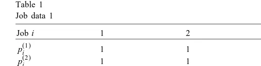
Table 1
operation followed – not necessarily immediately – by a specicoperation. These operations have processing times p(1)j and p(2)j , respectively. A set-up time is required before the rst standard operation and whenever there is a switch in production from specic to standard operations; two standard operations may be processed consecutively to form a batch without a set-up in between. With respect to the way in which standard operations are released (become available) after processing, two schemes are possible: batch availability, dened in Section 3, and the alternativeitem availabilitywhereby an operation becomes available immediately after it has been processed. We only analyze the batch availability variant explicitly and give comments as to how the result can be extended to the item availability case.
The model is introduced in [4] (for batch availability) and then analyzed for due-date related criteria in [10]. We note that the problem discussed in [4] for the sum of completion times objective was shown to be equivalent to the, seemingly simpler, problem studied in [7]. In particular, it was shown that the specic (unique) operations can essentially be removed from the problem. If this were also the case for the maximum lateness variants of these problems, then the results of Section 3 could be used directly to solve the problem discussed in this section. Before we proceed with our analysis, it is worthwhile to show that this is not the case. Consider the instance of the two-operation variant in which the set up time is c(c ¿0) and there are three jobs with due dates and operation processing times as shown in Table 1.
It can be easily veried that the problem of Section 3 obtained by omitting the specic operations, has as the unique optimal solution job 1 in the rst batch and jobs 2 and 3 in the second batch. The value of this solution is Lmax= 0. However, inserting the specic operations into this schedule (immediately after the
corresponding batch) yields a schedule for the two-component problem with lateness equal to c+ 4. It is easy to see that scheduling all the standard operations in one batch, followed by all the specic operations in EDD order, yields a schedule with lateness of 4. Thus, our example suggests that there is no obvious way to translate optimal solutions to the problem in Section 3 into optimal solutions for the problem in this section. This observation and the analysis below seem to lead to the conclusion that the problem in this section is genuinely more complex.
Returning to the two-operation problem, it is shown in [10] that there is an optimal schedule in which jobs complete according to the EDD rule. Thus, the jobs can be re-indexed according to this rule in O(nlogn) time and the problem reduces to one of batching that can be solved using a backward dynamic program with batch insertion [10]. LetGk denote the minimum overall lateness of a schedule containing jobsk; k+ 1; : : : ; n.
The initialization is Gn+1=−∞ and the recursion fork=n; n−1; : : : ;1 is
dynamic programming part can be implemented in O(nlogn) time thus yielding an overall time requirement of O(nlogn).
For the maximum in (8) to be given by the rst term, the following needs to hold:
Gl¿ max
for which (9) holds. We rst explain how we determine Ik−1
1 . Since the left-hand side value of (9) does not
depend on k and
Note that the right-hand side of (10) is a constant for xed k. Hence, if the inequality is satised for one or more indices in Ik
1, then these correspond to the smallest elements of the set {Gl−Pnh=lp
(2)
h |l∈ I1k}.
This fact can be used to eciently determine Ik−1
1 . In our implementation, we make use of a heap, which
we denote by H1. Recall that this data structure has the following properties [2]:
(i) the minimum of all values stored in the heap can be retrieved in constant time;
(ii) adding a value to the heap takes O(logm) time, wherem is the number of stored values; (iii) deleting the minimum value from the heap takes O(logm) time.
Suppose that heap H1 contains the values Gl−Pnh=lp
1 . To achieve this, we rst check whether the minimum value is less than the right-hand side of
(10). If this is the case, then we delete the minimum from H1 and we repeat the comparison with the new
minimum value. We keep deleting the current minimum value from H1 until this value becomes at least as
large as the right-hand side of (10) or until H1 is empty. Then we check whether Gk−Pnh=kp
of the indices that correspond to its elements.
Let us now turn to the issue of the ecient calculation ofGk. From the denition of I1k it follows that we
and
It follows that the minimum in (12) is attained for the smallest element of I2k, which we denote by qk; we
dene qk=k if I2=∅. Hence, (12) is equivalent to
From the discussion about the updating process of heapH1, it follows that the valuesqk are non-decreasing
in k. (Also note that keeping track of the values qk, k= 1;2; : : : ; n, requires overall O(n) time.) Hence, the
minimization is an instance of Problem P with uk=qk−1 and fj=−Pjh=1p (2)
h +dj. It follows that (12)
can be calculated for all values of k= 1;2; : : : ; n together in linear time.
For the ecient calculation of (11), we use a heapH2 which contains the valuesPl
−1 we simply retrieve the minimum from the heap. If the minimum corresponds to an element of I2k, we delete this value from H2 and retrieve the new minimum. This is repeated until the minimum corresponds to an
element of Ik
The time complexity of the above algorithm depends on the number of additions to and deletions from the heaps. For every l= 1;2; : : : ; n, the value Gl−Pnh=lp
h +Gl is added at most once to H2. (These additions actually occur at the same point
in time.) Furthermore, deletion from H1 and H2 also occurs at most once for every index. Since the heaps
never contain more than n elements, it follows that the total computational eort involving heap operations is O(nlogn).
We have now arrived at the required result: our algorithm solves the batching problem in O(nlogn) time thus yielding an overall time requirement of O(nlogn) time. This constitutes an improvement over the algorithm in [10].
Acknowledgements
Comments of an Associate Editor and an anonymous referee have improved the presentation of this paper. The authors wish to thank Chris Potts who suggested this research topic. Financial support by the Tinbergen Institute is gratefully acknowledged.
References
[1] A. Aggarwal, J.K. Park, Improved algorithms for economic lot size problems, Oper. Res. 41 (3) (1993) 549–571. [2] A.V. Aho, J.E. Hopcroft, J.D. Ullman, Data Structures and Algorithms, Addison-Wesley, Reading, MA, 1987. [3] S. Albers, P. Brucker, The complexity of one-machine batching problems, Disc. Appl. Math. 47 (1993) 87–107. [4] K.R. Baker, Scheduling the production of components at a common facility, IIE Trans. 20 (1) (1988) 32–35. [5] P. Brucker, Scheduling Algorithms, Springer, Berlin, 1995.
[6] P. Brucker, A. Gladky, H. Hoogeveen, M.Y. Kovalyov, C.N. Potts, T. Tautenhahn, S. van de Velde, Scheduling a batching machine, J. Schedul. 1 (1998) 31–54.
[7] E.G. Coman, M. Yannakakis, M.J. Magazine, C. Santos, Batch sizing and job sequencing on a single machine, Ann. Oper. Res. 26 (1990) 135–147.
[8] A. Federgruen, M. Tzur, A simple forward algorithm to solve general dynamic lot sizing models with nperiods in O(nlogn) or O(n) time, Manage. Sci. 37 (1991) 909–925.
[9] A.E. Gerodimos, C.A. Glass, C.N. Potts, Scheduling customised jobs on a single machine under item availability, unpublished report, Faculty of Mathematical Studies, University of Southampton, UK (1999).
[10] A.E. Gerodimos, C.A. Glass, C.N. Potts, Scheduling the production of two-operation jobs on a single machine, Euro. J. Oper. Res. 120 (2000) 250–259.
[11] M.Y. Kovalyov, C.N. Potts, Scheduling with batching: a review, Euro. J. Oper. Res. 120 (2000) 228–249.
[12] C.A. Santos, M.J. Magazine, Batching in single operation manufacturing systems, Oper. Res. Lett. 4 (3) (1985) 99–103.
[13] S. van Hoesel, A. Wagelmans, B. Moerman, Using geometric techniques to improve dynamic programming algorithms for the economic lot-sizing problem and extensions, Euro. J. Oper. Res. 75 (1994) 312–331.
[14] A. Wagelmans, S. van Hoesel, A. Kolen, Economic lot sizing: an O(nlogn) algorithm that runs in linear time in the Wagner–Whitin case, Oper. Res. 40 (Supp. 1) (1992) 145–156.