SEA SURFACE ALTIMETRY BASED ON AIRBORNE GNSS SIGNAL MEASUREMENTS
K. Yu, C. Rizos, A. Dempster
School of Surveying and Spatial Information Systems, University of New South Wales, Sydney, NSW 2052, Australia (kegen.yu, c.rizos, a.dempster)@unsw.edu.au
KEY WORDS: Sea Surface Altimetry, GNSS Reflectometry, Airborne Experiment, LiDAR Measurement
ABSTRACT:
In this study the focus is on ocean surface altimetry using the signals transmitted from GNSS (Global Navigation Satellite System) satellites. A low-altitude airborne experiment was recently conducted off the coast of Sydney. Both a LiDAR experiment and a GNSS reflectometry (GNSS-R) experiment were carried out in the same aircraft, at the same time, in the presence of strong wind and rather high wave height. The sea surface characteristics, including the surface height, were derived from processing the LiDAR data. A two-loop iterative method is proposed to calculate sea surface height using the relative delay between the direct and the reflected GNSS signals. The preliminary results indicate that the results obtained from the GNSS-based surface altimetry deviate from the LiDAR-based results significantly. Identification of the error sources and mitigation of the errors are needed to achieve better surface height estimation performance using GNSS signals.
1. INTRODUCTION
GNSS-R is a promising technique that can be exploited to remotely sense a range of geophysical parameters, as originally proposed by Martin-Neira (1993). One specific application area of GNSS-R is sea surface altimetry. Compared to radar altimetry, GNSS altimetry is able to provide much larger data coverage due to the fact that the airborne or spaceborne receiver can receive signals transmitted from multiple GNSS satellites and reflected over a large sea surface area. The current radar altimeters are not able to measure mesoscale processes that are the dominant error source in global climate modelling, while GNSS altimetry provides a potential and inexpensive way to measure such processes. A quite comprehensive treatment of the theory of GPS-based ocean altimetry is provided by Hajj and Zuffada (2003). Also, a number of experiments under different scenarios were conducted by researchers and reported in the literature. GPS altimetry experiment over a lake was carried out by Treuhaft et al (2001). Bridge-based experiments were reported by Rius et al (2011). Airborne experiments were carried out and reported by Lowe et al (2002) and Rius et al
(2010). Results of ESA’s spaceborne PARIS experiments and altimeter in-orbit demonstrator were reported by Martin-Neira
et al (2011).
In this paper we investigate sea surface altimetry using GNSS signals. One study is how the altimetry performance is affected by the surface roughness, especially when the surface wave height is rather high, owing to strong local wind and/or swells. A low-altitude airborne experiment was conducted in June 2011 by a UNSW-owned light aircraft flying off the coast of Sydney when the sea surface was rather rough. A LiDAR experiment was conducted in the same aircraft, whose first objective was to monitor the Sydney coastal areas to provide information for future infrastructure development; and the second one was to estimate the sea surface height as a reference to the results generated from the GNSS-based altimetry. A two-loop iterative method is proposed to estimate the surface height using the arrival time difference between the direct and reflected GNSS signals. This method is comparatively simple and can be readily implemented. Through processing the experimental data it is
demonstrated that the LiDAR data not only can serve as a reference for mean sea level (MSL), but they also provide the statistics of the sea surface roughness, including the significant wave head (SWH), the root-mean-square (RMS) wave height, and the maximum wave height. Note that there are a significant number of reports in the literature on using LiDAR for sea surface topography (Reineman et al 2009 and Vrbancich et al
2011). It is observed that there is good agreement between the wave head statistics calculated from the LiDAR data and those obtained from a Waverider buoy. In the case of GNSS-based altimetry, some preliminary results are produced. Compared to the results obtained from the LiDAR data, the estimation error associated with the GNSS-based method is large. Finding the error sources and mitigating the estimation errors is the topic of ongoing work.
The remainder of the paper is organised as follows. The following section presents the basic theory of GNSS-based altimetry and describes a two-loop iterative method for calculating surface height. Section 3 describes the airborne GNSS experiment and the LiDAR experiment. Section 4 presents experimental and estimation results, and Section 5 concludes the paper.
2. GNSS-BASED SEA SURFACE ALTIMETRY 2.1 Fundamentals
The principle of the GNSS altimetry is quite simple, as illustrated in Figure 1. The receiver may be either on an airborne or on a spaceborne platform, and receives the signals transmitted by three GNSS satellites and reflected by the water or ice surface. Depending on the surface roughness each signal may be reflected at many surface points and received by the receiver via the down-looking antenna. However, the surface point of interest is the specular point from which the signal propagation path length is the minimum. The sea surface height is calculated by measuring the delay of the direct signal and that of the reflected signal. The delay or code phase of the direct signal can be readily determined by cross-correlating the received signal with a code (C/A-code or P-code) replica. The ISPRS Annals of the Photogrammetry, Remote Sensing and Spatial Information Sciences, Volume I-7, 2012
delay is simply estimated as the time point where the cross-correlation reaches the maximum. On the other hand the determination of the delay of the reflected signal can be more complex. In the case where the receiver altitude is very low such as around tens of metres, the method used for direct signals can be directly applied to reflected signals (Martin-Reina 2001). It is a fact that due to surface roughness the delay of the specular reflection point does not correspond to the peak of the cross-correlation. However, at such low altitudes, the roughness-induced error is smaller than the observation noise hence it can be ignored. As for airborne altimetry a few kilometres or spaceborne altimetry of several hundreds of kilometres above the sea, the displacement between time point of the peak of the cross-correlation and that of the delay can be significant. To determine the true delay of the signal reflected at the specular point, the derivative of the delay waveforms can be exploited (Hajj & Zuffada 2003, Rius et al 2010). That is, the time point of the peak of the derivative of the waveform corresponds to the delay of the reflected signal.
Figure 1: Principle of GNSS altimetry
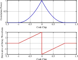
In the case of an ideally perfect smooth sea surface, the reflected signals would have a triangle correlation function which is the same as the direct signals. Thus the reflected signal has a delay waveform and its derivative as illustrated in Figure 2. In this idealised case the delay of the reflected signal can be readily determined either from the delay waveform or from the derivative of the waveform.
-1.50 -1 -0.5 0 0.5 1 1.5
Figure 2. Delay waveform and its derivative of a GNSS signal reflected from a perfectly smooth sea surface.
The upper plot of Figure 3 shows the delay waveform that is generated using data logged during an airborne experiment. The sampling frequency of the IF data is 16.3676MHz, corresponding to a resolution of 18.33 metres, which is too large in terms of sea surface altimetry. Thus interpolation of the samples is required to obtain a much higher resolution. From the upper plot in Figure 3 the effect of the interpolation can be readily observed. The post-interpolation delay waveform was produced using the Matlab library function “INTERP”. The
derivative of the post-interpolation delay waveform is shown in the lower plot of Figure 3. In this case the displacement between the peak of the waveform and the peak of the derivative of the waveform is 0.2233 code chips, corresponding to 218.24 nanoseconds or 65.47 metres.
2.4 2.45 2.5 2.55 2.6 2.65
Figure 3. Interpolation of delay waveform (top) and derivative of delay waveform (bottom).
Since the position of the GNSS satellite is known and the position of the receiver can be determined using the direct signals associated with such as eight or even more satellites, the distance between the GPS satellite and the receiver can be receiver and the satellite, respectively. Thus with the knowledge of the relative delay (rd) of the reflected signal with respect to
the direct signal, the total distance (RtSr) from the GNSS transmitter through the specular reflection point and to the receiver can be readily determined as:
rd tr tSr R c
Rˆ ˆ (2)
where c is the propagation speed of light and ˆrd is the estimate of rd. As a consequence the position of the specular reflection point on the sea surface can be calculated by solving the point on the sea surface.
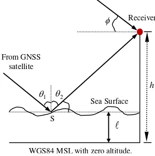
In Figure 4 point S is the specular reflection point in the rough sea surface, whose altitude over the WGS84 MSL is to be estimated. The actual sea surface can be significantly different the WGS84 MSL where the altitude is defined as zero, although the difference of the surfaces (actual sea surface, MSL and geoid) is ignored in some cases. A number of notations or symbols in the figures are defined as:
= satellite elevation angle at the receiver
2 1,
= incident angle at specular point S
h = WGS84 altitude of the receiver
= distance from specular point S to the WGS84 MSL GNSS SAT#1
2.2 Proposed Iterative Method
Clearly the aim is to determine the parameter and a two-loop iterative method is proposed here to solve the problem. Specifically the inner loop is for calculating the position of the specular point S, while the outer loop is for selecting the surface height. Initially, a guess of the sea surface height is given based on some prior information about the surface height in the area of interest. In the event that there is no relevant prior information, the initial value may be simply set at zero, i.e. the specular point is assumed to be on the surface of the WGS84 geoid surface where the altitude is zero. For a given surface height, say ~, the coordinates of the specular point can be determined by minimising the total path length defined by (3). Then the minimum path length (R~tSr) is compared with the
measured actual path length (RˆtSr) given by (2). If R~tSrRˆtSr,
then the tentative surface height is increased by an increment. Otherwise, it is decreased. The procedure continues until the difference between the two path lengths is sufficiently small. To reduce the computational complexity, a simple technique may
be used. For instance, if RtSr RˆtSr
~
, the tentative surface height is increased by a relatively larger increment such as 40 metres.
At the next iteration of the outer loop if R~tSrRˆtSr, the
increment is decreased by half of the previous increment. In this way, the process will quickly converge to the steady state.
Note that the specular reflection must satisfy Snell’s Law, i.e. the two angles (1 and 2 in Figure 4) between the incoming
wave and the reflected wave, separated by the surface normal must be equal. Thus the results should be tested to see if this Law is satisfied.
Figure 4. Geometry of the receiver, WGS84 mean sea level, rough sea surface, direct and reflected signal paths.
A method for determining the specular point on the WGS84 surface with a zero altitude can be found in Gleason (2009). Here the modified version of the method is given to accommodate the non-zero altitude value. From (3) the partial derivatives with respect to the coordinates of the specular point can be determined as:
, S { S, S, S}
which can be rewritten in a vector form as:
tS point, the receiver and the transmitter, respectively. Equation (4) is the basis to generate an iterative solution to the minimum path length. That is, at time instant n1 the specular point position is updated according to:
S
where is a constant which typically should be set as a larger value as the flight altitude increases. The initial guess of the specular point position is scaled according to:
|
where the radius of the Earth at the specular point is calculated by: estimate of the mean sea surface height. However, a reasonable estimate of the mean surface height will be produced through the generation and subsequent processing of the altitude estimates of many specular points over a period of time.
3. LOW-ALTITUDE AIRBORNE EXPERIMENT A low-altitude airborne experiment was conducted by a UNSW-owned light aircraft off the coast of Sydney between Narrabean Beach and Palm Beach on the 14th of June 2011. Both the LiDAR experiment and the GNSS-R experiment were carried in the same aircraft at the same time. Due to the requirement of the LiDAR experiment, the aircraft flight height was below 500 device is extremely rugged and thus ideally suited for airborne experiment. The maximum measurement range is around 650m and ranging accuracy is about 20mm.
The LHCP (light hand circularly polarised) and RHCP (right hand circularly polarised) antennas and the low noise amplifier (LNA) are also secured either on the top or on the bottom of the aircraft as shown in Figure 7. The direct signal was captured via
h
WGS84 MSL with zero altitude. Receiver
the zenith-looking RHCP antenna, whereas the reflected signal was received via the nadir-looking LHCP antenna. Both signals were processed through the software receiver, which has four RF front-ends to generate the IF signals that were logged to a laptop for subsequent processing.
Figure 5. Light aircraft used for conducting the experiment.
Figure 6. GPS software receiver (left front) and LiDAR equipment (rear) secured in the aircraft.
Figure 7. RHCP antenna (left), LHCP antenna (middle) and low noise amplifier (right).
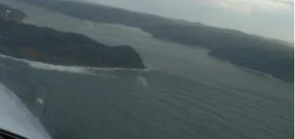
The wind and wave conditions during the experiment day are shown in Figures 8 and 9, respectively. The wind data were provided by the Australian Bureau of Meteorology, while the wave data were provided by Mark Kulmar from the Manly Hydraulics Laboratory, Sydney, New South Wales. It can be seen that the wind was strong with speeds between 7.2m/s (26km/h) and 13.9m/s (or 50km/h). The sea surface was rather rough with the SWH (significant wave height) between 2.65m and 4.18m and the maximum wave height was greater than 6m. Figure 10 shows the sea surface conditions viewed from the aircraft.
9 10 11 12 13 14 15 16 17
0 5 10 15 20 25
Time (am & pm)
W
in
d
S
p
e
e
d
a
n
d
G
u
st
(m
/s
)
9 10 11 12 13 14 15 16 17
0 50 100 150
Time (am & pm)
W
in
d
D
ire
c
ti
o
n
(d
e
g
)
Gust Speed
Figure 8. Wind speed and direction during the day when the experiments were conducted.
9 10 11 12 13 14 15 16 17
2 4 6 8
Time (am & pm)
W
a
v
e
H
e
ig
h
ts
(m
)
9 10 11 12 13 14 15 16 17
2 4 6 8 10
Time (am & pm)
W
a
v
e
P
e
ri
o
d
ss
(s
e
c
)
SWH RMS wave height maximum wave height
zero crossing period significant period period of waves with most energy
Figure 9. Wave heights and periods during the day when the experiments were conducted.
Figure 10. Sea surface conditions viewed from the aircraft.
4. EXPERIMENTAL RESULTS 4.1 LiDAR Experimental Results
Figure 11 shows the results related to 3983 points on the sea surface from processing of the LiDAR data. The upper plot shows the WGS84 altitudes of the surface points and their mean (dashed straight line), while the lower plot shows the difference when the altitudes are subtracted by the mean of the altitudes. That is, the lower plot shows the surface elevation variation with respect to the measured MSL which is calculated as 23.444m. The standard deviation of the MSL estimate is 1.38metres, mainly contributed to by the surface roughness. This MSL estimate can be employed as a reference when evaluating the performance of the GNSS-based altimetry. These samples were taken between 15:27:55 and 15:31:38, for duration of 3 min 43.3 sec. The Waverider buoy-based wave height measurements (see Figure 9) indicate that during this period the SWH, RMS (root mean square) wave height, and maximum wave height were 4.0m, 2.7m, and 6.4m, respectively. Figure 12 shows the wave heights derived from the LiDAR surface points shown in Figure 11. A wave is defined as the portion of the water between two successive zero-up-crossings relative to the MSL. The wave height is simply calculated as the vertical displacement between the crest and the trough of the wave. Using these LiDAR-based wave heights the SWH, RMS wave height, and maximum wave height are calculated as 3.72m, 2.61m, and 6.78m, respectively. It can be seen that these LiDAR-based statistics of the wave height measurements have good agreement with those of the Waverider buoy-based measurements. Note that the distance between the location of the Waverider buoy and the location where the presented data were collected is between 10.45km and 12.50km. Due to this location difference some small variations of the wave statistics are expected. Figure 14 shows the cumulative distribution function (CDF) of the measured wave heights. It can be seen that the measured wave heights closely follow the Rayleigh distribution whose CDF is given by ISPRS Annals of the Photogrammetry, Remote Sensing and Spatial Information Sciences, Volume I-7, 2012
))} (Longuet-Higgins 1952, Dean & Dalrymple l991).
0 0.5 1 1.5 2 2.5 3 3.5
Figure 11. WGS84 altitudes of the sea surface points (top) and relative sea surface elevation (bottom) measured by LiDAR.
50 100 150 200 250 300 350 400
Figure 12. Wave heights derived from the LiDAR surface points.
Figure 13. Cumulative distribution functions of the measured wave heights and the Rayleigh variable.
4.2 GNSS-R Experimental Results
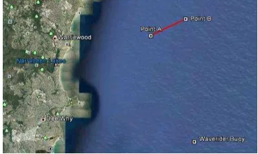
Figure 14 shows the short flight track segment relative to the coastal area over the duration of about 50 seconds. The distances between the Waverider buoy and the two points A and B are RAB2.98 km, RAW8.97 km, and RBW9.54 km,
respectively. The satellites with elevation angles greater than 40 degrees are listed in Table 1, where two angle values are for points A and B respectively. Since the duration is just 50 seconds, the elevation angle of each satellite changes little. Figure 15 shows the flight height and the aircraft speeds over the duration of 50 seconds. The flight height was just around 300 metres, equivalent to about one C/A (coarse/acquisition) code chip. The C/A code is a deterministic sequence of 1023 bits, which is called pseudorandom noise (PRN) code. Each
GNSS satellite is assigned with one specific PRN code with a unique code number to distinguish from each other.
Figure 14. Experimental location. The data collected over 50 seconds between points A and B.
Table 1. Satellite elevation angles (deg) at Points A and B.
Satellite 22 18 6 21 14
Figure 15. Aircraft altitude and speed over the duration of 50 seconds.
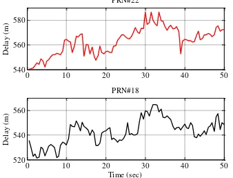
Figure 17 shows the delay estimates of the reflected signal relative to the direct signal associated with two satellites (PRN#22 and PRN#18). The delays were estimated based on the delay waveforms of the direct and reflected signals as mentioned earlier. The waveforms were produced by coherent integration of the received signals over 1 millisecond and then combined through non-coherent integration over 1 second. Over the period of 50 seconds, the relative delay varies significantly. Ongoing work will focus on why the relative delay changes so much. Certainly, the surface roughness will affect the delay estimation, but the impact should not be so much. Figure 18 shows the sea surface height estimates associated with the two satellites. The means of the estimates are 18.6 metres and 15.4 metres respectively, while the standard deviations are 7.41 metres and 7.04 metres respectively. Clearly, the estimation results do not have good agreement with the results provided by the LiDAR experiment. This will be the subject of further investigation. A number of factors may contribute to such an outcome. The surface roughness is one, as already mentioned. The second factor may be the delay estimation error, and another factor is that we have not performed a careful calibration for the relative positions of the zenith-looking antenna and the nadir-looking antenna. Further, the number of samples used for the estimation may not be sufficient. To ISPRS Annals of the Photogrammetry, Remote Sensing and Spatial Information Sciences, Volume I-7, 2012
achieve accurate surface altimetry, all these issues need to be considered.
0 10 20 30 40 50
540 560 580
D
e
la
y
(
m
)
PRN#22
0 10 20 30 40 50
520 540 560
Time (sec)
D
e
la
y
(
m
)
PRN#18
Figue 16. Delay of the reflected signal relative to the direct signal associated with two satellites.
0 10 20 30 40 50
0 20 40
A
lt
it
u
d
e
E
st
im
a
te
(
m
) PRN#22
0 10 20 30 40 50
0 20 40
Time (sec)
A
lt
it
u
d
e
E
st
im
a
te
(
m
) PRN#18
Figure 17. Surface height estimates using signals associated with two satellites (PR#22 and PRN#18).
5. CONCLUDING REMARKS
In this paper we investigated sea surface height estimation based on GNSS signal measurements. A LiDAR experiment and a GNSS-R experiment were conducted in the same aircraft at the same time. By processing the data obtained from the LiDAR experiment, the statistics of the wave heights were produced, showing good agreement with the results obtained from a nearby Waverider buoy. Information about the sea surface height was also derived from the LiDAR data. GNSS-based surface height estimation was performed by estimating the relative delay between the direct and the reflected signals. A two-loop iterative method was proposed to calculate the surface height. The results obtained from the GNSS altimetry did not have good agreement with the LiDAR-based results. Ongoing work will focus on finding the error sources and improving the estimation accuracy.
ACKNOWLEDGEMENTS
The authors would like to acknowledge that this research work was carried out for the SAR Formation Flying Project which was funded by the Australian Space Research Program (ASRP) and for the ARC Discovery Project DP0877381 (Environmental Geodesy: Variations of Sea Level and Water Storage in the Australian Region). The authors would also like to thank their colleagues Mr. Peter Mumford, Mr. Greg Nippard and Prof. Jason Middleton for conducting the airborne experiments.
REFERENCES
Dean, R.G. and Dalrymple, R.A., 1991. Water Wave Mechanics for Engineers andScientists,World Scientific, Singapore.
Gleason, S.T., Gebre-Egziabher, D., 2009. GNSS Applications and Methods, Artech House.
Hajj, G.A. and Zuffada, C., 2003. Theoretical description of a bistatic system for ocean altimetry using the GPS signal, Radio Science, 38(5), pp. 1-10.
Longuet-Higgins, M.S., 1952. On the statistical distribution of the heights of sea waves, Journal of Marine Research, 11(3), pp. 245-266.
Lowe, S.T., Zuffada, C., Chao, Y., Kroger, P., LaBrecque, J., Young, L.E., 2002. 5-cm-precision aircraft ocean altimetry using GPS reflections, Geophysical Research Letters, 29(10), 13.1-13.4.
Martín-Neira, M., 1993. A passive reflectometry and interferometry system (PARIS): Application to ocean altimetry,
ESA Journal, 17(14), pp. 331–355.
Martin-Neira, M., Caparrini, M., Font-Rossello, J., Lannelongue, S., Vallmitjana, C.S., 2001. The PARIS concept: An experimental demonstration of sea surface altimetry using GPS reflected signals, IEEE Transactions on Geoscience and Remote Sensing, 39(1), 142-150.
Reineman, B.D., Lenain, L., Melville, W.K., 2009. A portable airborne scanning Lidar system for ocean and coastal applications. Journal of Atmospheric and oceanic technology, 26(12), 2626-2641.
Rius, A., Cardellach, E., Martın-Neira, M., 2010. Altimetric analysis of the sea-surface GPS-reflected signals. IEEE Transactions on Geoscience and Remote Sensing, 48(4), 2119– 2127.
Rius, A., Nogues-Correig, O., Ribo, S., Cardellach, E., Oliveras, S., Valencia, E., Park, H., Tarongi, J.M., Camps, A., Marel, H.V.D., Bree. R.V., Altena, B., Martin-Neira, M., 2011. Altimetry with GNSS-R interferometry: First proof of concept experiment, GPS Solutions, DOI 10.1007/s10291-011-0225-9.
Treuhaft, R., Lowe, S.T., Zuffada, C., Chao, Y., 2001. 2-cm GPS altimetry over Crater Lake, Geophysical Research Letters, 28(23), 4343-4346.
Vrbancich, J., Lieff, W., Hacker,J, 2011. Demonstration of two portable scanning LiDAR systems flown at low-altitude for investigating coastal sea surface topography. Remote Sensing, 3(9), 1983-2001.