Full Terms & Conditions of access and use can be found at
http://www.tandfonline.com/action/journalInformation?journalCode=ubes20
Download by: [Universitas Maritim Raja Ali Haji] Date: 12 January 2016, At: 17:49
Journal of Business & Economic Statistics
ISSN: 0735-0015 (Print) 1537-2707 (Online) Journal homepage: http://www.tandfonline.com/loi/ubes20
VARMA versus VAR for Macroeconomic Forecasting
George Athanasopoulos & Farshid Vahid
To cite this article: George Athanasopoulos & Farshid Vahid (2008) VARMA versus VAR for Macroeconomic Forecasting, Journal of Business & Economic Statistics, 26:2, 237-252, DOI: 10.1198/073500107000000313
To link to this article: http://dx.doi.org/10.1198/073500107000000313
Published online: 01 Jan 2012.
Submit your article to this journal
Article views: 198
View related articles
VARMA versus VAR for
Macroeconomic Forecasting
George A
THANASOPOULOSDepartment of Econometrics and Business Statistics, Monash University, Clayton, Victoria 3800, Australia (George.Athanasopoulos@buseco.monash.edu.au)
Farshid V
AHIDSchool of Economics, Australian National University, Canberra, ACT, 0200, Australia
In this article, we argue that there is no compelling reason for restricting the class of multivariate models considered for macroeconomic forecasting to vector autoregressive (VAR) models, given the recent ad-vances in vector autoregressive moving average (VARMA) modeling methodology and improvements in computing power. To support this claim, we use real macroeconomic data, and show that VARMA models forecast macroeconomic variables more accurately than VARs.
KEY WORDS: Identification; Multivariate time series; Scalar components; VARMA models.
1. INTRODUCTION
Finite-order vector autoregressive moving average (VARMA) models are motivated by the Wold decomposition theorem (Wold 1938) applied in a multivariate setting, as an appropri-ate class of models for stationary time series. Hence, the study of VARMA models has been an important area of time series analysis for a long time (see, among others, Quenouille 1957; Hannan 1969; Tunnicliffe-Wilson 1973; Hillmer and Tiao 1979; Tiao and Box 1981; Tiao and Tsay 1989; Tsay 1991; Poskitt 1992; Lütkepohl 1993; Lütkepohl and Poskitt 1996; Reinsel 1997; Tiao 2001). However, macroeconomists have yet to be convinced of the advantages of employing such models. One of the reasons might be that, to date, no applied macro-econometric research paper has considered the VARMA model as an alternative to the finite-order vector autoregressive (VAR) model.
Ever since the publication of the seminal paper by Christo-pher Sims (Sims 1980), the finite-order VAR model has become the cornerstone of macroeconometric modeling. The reason for this cannot be that economic theory implies finite-order VAR dynamics for economic variables. Economic theory rarely has any sharp implications about the short-run dynamics of eco-nomic variables. In the rare situations where theoretical models include a dynamic adjustment equation, one has to work hard to exclude moving average terms from appearing in the implied dynamics of the variables of interest. Even if we believe that a finite-order VAR is a good dynamic model for a particular set of variables, for any subset of these variables, a VARMA model rather than a VAR model would be appropriate. Therefore, the apparent lack of interest in multivariate models with moving average errors could be either because they are too difficult to implement, or because pure autoregressive models can perform just as well.
Any invertible VARMA process can be approximated by a finite long-order VAR. However, this does not imply that fore-casts based on an estimated long-order VAR will be as good as those based on a parsimonious VARMA model, because a long-order VAR has many estimated parameters. It appears that the main reason for the lack of enthusiasm for using models with moving average errors is that they are too difficult. In particu-lar, in a multivariate setting, the identification and estimation of
VARMA models are quite involved. This is in sharp contrast to the ease of identification and estimation of VAR models. This difficulty in model identification and estimation has thus far deterred any comprehensive assessment of whether VARMA models outperform VAR models in forecasting macroeconomic variables in finite samples.
Theoretically, there is no subtlety involved in the estimation of an identifiedVARMA(p,q)model. Based on the assumption of normality, the likelihood function, conditional on the firstp observations being fixed and theqerrors before timep+1 being set to zero, is a well-defined function that can be calculated re-cursively. The exact likelihood function can also be computed via the Kalman filter after the model has been written in its state space form. However, it is not possible to fit a “general”
VARMA(p,q)model to any set of observations, and then to try
and reduce the system to a more parsimonious one by eliminat-ing the insignificant parameters. The reason for this is that if the parameters of aVARMA(p,q)model satisfy certain restrictions, the model will not be identified. The following simple example illustrates this point.
Example 1. Consider the following bivariate VARMA(1,1)
process:
y1,t=φ11y1,t−1+φ12y2,t−1+θ11η1,t−1
+θ12η2,t−1+η1,t,
(1) y2,t=φ21y1,t−1+φ22y2,t−1+θ21η1,t−1
+θ22η2,t−1+η2,t.
This model is not identified if φ21=φ22=θ21=θ22=0. In this case the second equation implies thaty2,t−1=η2,t−1, and thereforeφ12andθ12 in the first equation cannot be identified separately.
There are several methods for identifying VARMA models. The method that we consider in this article is the Athanasopou-los and Vahid (2006) extension to Tiao and Tsay (1989). This
© 2008 American Statistical Association Journal of Business & Economic Statistics April 2008, Vol. 26, No. 2 DOI 10.1198/073500107000000313
237
methodology consists of three stages. In the first stage, “scalar component models” (SCMs) embedded in the VARMA model are identified using a series of tests based on canonical correla-tions analysis between judiciously chosen sets of variables. In the second stage, a fully identified structural form is developed through a series of logical deductions and additional canonical correlations tests. Then in the final stage, the identified model is estimated using full information maximum likelihood (FIML). An overview of this methodology is presented in Section 2. In this article we employ this methodology to answer the question of whether VARMA models outperform VAR models in fore-casting macroeconomic variables.
To compare the forecasting performance of VARMA and VAR models, we use real data. As a first example, we com-pile many trivariate sets of monthly macroeconomic variables and choose 50 in which VARs forecast better than univariate ARs. We fit VAR and VARMA models to them, using only one portion of the available sample for estimation and holding the rest of the sample for a forecast comparison. Using the esti-mated models, we forecast these variables 1 to 15 steps into the future throughout the forecast period. We then use several mea-sures of forecast accuracy to compare the performance of the VARMA and VAR models. In another example, we use quar-terly U.S. GDP growth, inflation, short-term interest rate, and the term spread. These four macroeconomic variables have fea-tured prominently in the recent empirical literature. We com-pare the performance of VARMA, VAR, and univariate AR models in forecasting these variables. Finally, taking the esti-mated VARMA model for these four variables as a base data generating process, we perform a Monte Carlo analysis and explore what feature of the data is most responsible for the better forecasting performance of VARMA models relative to VARs.
In practice, VAR models are used not only for forecast-ing, but also for impulse response and variance decomposition analysis. However, because the true model is not known, it is not possible to use real data to compare the performance of VARMA versus VAR models in tasks other than forecasting. Comparisons of impulse responses and variance decomposi-tions can only be performed when the data generating process is known. However, because of the large dimension of the pa-rameter space in multivariate time series models, designing a Monte Carlo study that is sufficiently rich to lead to convincing general conclusions would be difficult, if not impossible. For this reason, we use real macroeconomic data for this investiga-tion, and compare the out-of-sample forecasting performance of fitted VARMA and VAR models. The advantage of this method is that the results will be of direct relevance for macroeconomic forecasting. The drawback is the inability to assess or comment on which model produces a better impulse response function or a better decomposition of the forecast error variance, because these objects of interest are not observable.
The structure of the article is as follows. Section 2 outlines our VARMA modeling methodology. Section 3 describes the forecast evaluation method and presents the results of three methods of investigating if and why VARMA models produce better forecasts than VAR models. Section 4 provides some con-clusions.
2. A VARMA MODELING METHODOLOGY BASED
ON SCALAR COMPONENTS
The VARMA modeling methodology we employ in this arti-cle is the Athanasopoulos and Vahid (2006) extension to Tiao and Tsay (1989). In this section we present a brief overview of the methodology. For more details, readers should refer to the above-mentioned articles.
The aim of identifying scalar components is to examine whether there are any simplifying embedded structures under-lying aVARMA(p,q)process.
Definition 2. For a givenK-dimensionalVARMA(p,q)
pro-cess
yt=1yt−1+ · · · +pyt−p+ηt
−1ηt−1− · · · −qηt−q, (2) a nonzero linear combinationzt=α′ytfollows anSCM(p1,q1) ifαsatisfies the following properties:
α′p1=0
Notice that the scalar random variablezt depends only on lags 1 top1of all variables, and lags 1 toq1of all innovations in the system. Tiao and Tsay (1989) employed a sequence of canonical correlations tests to discoverKsuch linear combina-tions.
Denote the squared sample canonical correlations between
Ym,t ≡(y′t, . . . ,y′t−m) and Yh,t−1−j ≡(y′t−1−j, . . . ,y′t−1−j−h)′ byλ1<λ2<· · ·<λK. The test statistic suggested by Tiao and Tsay (1989) for testing for the null of at least s SCM(pi,qi) against the alternative of fewer thansscalar components is
C(s)= −(n−h−j) wherediis a correction factor that accounts for the fact that the canonical variates in this case can be moving averages of order j. Specifically,
whereρv(·)is thevth-order autocorrelation of its argument and
r′iYm,t andg′iYh,t−1−j are the sample canonical variates cor-responding to theith canonical correlation betweenYm,t and
Yh,t−1−j.
Suppose we haveKlinearly independent scalar components characterized by the transformation matrixA=(α1, . . . ,αK)′. If we rotate the system in(2)byA, we obtain
Ayt=1yt−1+ · · · +pyt−p+εt
−∗1εt−1− · · · −∗qεt−q, (4)
wherei=Ai,εt=Aηt, and∗i =AiA−1,in which the right-side coefficient matrices have many rows of zeros. How-ever, as the following simple example shows, even if A is known, there are still situations where the system is not iden-tified.
Example 3. Consider the bivariateVARMA(1,1)system with
two scalar componentsSCM(1,1)andSCM(0,0), that is, The second row of the system implies that
a21y1,t−1+a22y2,t−1=ε2,t−1.
y1,t−1,y2,t−1, andε2,t−1all appear in the right side of the first equation of the system and therefore their coefficients are not identified. We setθ12(1)=0 to achieve identification.
In general, if there exist two scalar componentsSCM(pr,qr) andSCM(ps,qs), where pr>ps andqr >qs, the system will not be identified. In such cases min{pr−ps,qr −qs} autore-gressive or moving average parameters must be set to zero for the system to be identified. This is referred to as the “general rule of elimination” (Tiao and Tsay 1989). The methodology we employ here requires us to set the moving average parame-ters to zero in these situations (see Athanasopoulos and Vahid 2006, for a more detailed explanation).
Tiao and Tsay (1989) constructed a consistent estimator for
A using the estimated canonical covariates corresponding to insignificant canonical correlations. Conditional on these esti-mates, they estimated the row sparse parameter matrices on the right side of (2). The lack of proper attention to efficiency in the estimation ofA, which affects the accuracy of the second-stage estimates, was a major criticism of the Tiao and Tsay method-ology raised by many eminent time series analysts (see the dis-cussion by Chatfield, Hannan, Reinsel, and Tunnicliffe-Wilson that followed Tiao and Tsay 1989).
The Athanasopoulos and Vahid (2006) extension to the Tiao and Tsay (1989) methodology concentrated on establishing necessary and sufficient conditions for the identification of A
such that all parameters of the system can be estimated simul-taneously using FIML (Durbin 1963, 1988). These rules are:
1. Each row ofAcan be multiplied by a constant without changing the structure of the model. Hence, we are free to normalize one parameter in each row to 1. However, as always in such situations, there is the danger of choos-ing a parameter whose true value is zero for normaliza-tion, that is, a zero parameter might be normalized to 1. To safeguard against this, the procedure adds tests of pre-dictability using subsets of variables. Starting from the SCM with the smallest order (the SCM with minimum p+q), exclude one variable, say the Kth variable in a K-dimensional system, and test whether an SCM of the same order can be found using theK−1 variables alone. If the test is rejected, the coefficient of the Kth variable is then normalized to 1 and the corresponding coefficients in all other SCMs that nest this one are set to zero. If the
test concludes that the SCM can be formed using the first K−1 variables only, the coefficient of theKth variable in this SCM is zero, and should not be normalized to 1. It is worth noting that if the order of this SCM is uniquely minimal, then this extra zero restriction adds to the re-strictions discovered before. Continue testing by omitting variableK−1 and test whether the SCM could be formed from the firstK−2 variables only, and so on.
2. Any linear combination of an SCM(p1,q1) and an
SCM(p2,q2)is anSCM(max{p1,p2},max{q1,q2}). In all cases where there are two embedded scalar components with weakly nested orders, that is,p1≥p2 andq1≥q2, arbitrary multiples of SCM(p2,q2)can be added to the
SCM(p1,q1)without changing the structure of the sys-tem. This means that the row ofAcorresponding to the SCM(p1,q1)is not identified in this case. To achieve iden-tification, if the parameter in theith column of the row of
Acorresponding to theSCM(p2,q2)is normalized to 1, the parameter in the same position in the row ofA corre-sponding toSCM(p1,q1)should be restricted to zero.
A brief summary of our complete VARMA methodology is as follows.
Stage I: Identification of the Scalar Components
This stage follows the Tiao and Tsay (1989) methodology and comprises two steps:
Step 1: Determining an Overall Tentative Order. Starting
fromm=0,j=0 and incrementing sequentially one at a time, find all zero sample canonical correlations between Ym,t and
Ym,t−1−j. Organize the results in a two-way table. Starting from the upper left corner and considering the diagonals perpendicu-lar to the main diagonal (i.e., the trailing diagonals), search for the first time thats+K zero eigenvalues are found, given that there are s zero eigenvalues in position(p−1,q−1)(when eitherp=1 orq=1,s=0). This(p,q)is taken as the overall order of the system. Note that it is possible to find more than one such(p,q)and therefore more than one possible overall order. In such cases, one should pursue all of these possibilities and choose between competing models using a model selection cri-terion. The maximum order we test for in the empirical section that follows is max(p,q)=(4,4). (This procedure produces ex-actly the same results as those implied by the “Criterion Table” in Tiao and Tsay 1989.)
Step 2: Identifying Orders of SCMs. Conditional on(p,q),
test for zero canonical correlations between Ym,t and
Ym+(q−j),t−1−j for m=0, . . . ,p and j=0, . . . ,q. Note that because an SCM(m,j) nests all scalar components of order (≤m,≤j), for every one SCM(p1<p,q1<q) there will be
s=min{m−p1+1,j−q1+1}zero canonical correlations at position(m≥p1,j≥q1). Therefore, for every increment above
s, a new SCM(m,j)is found. This procedure does not neces-sarily lead to a unique decision about the embedded SCMs. In all such cases, all possibilities should be pursued and the final models can be selected based on a model selection criterion. (The tabulation of all zero eigenvalues produces the “Root Ta-ble” of Tiao and Tsay 1989.)
Stage II: Placing Identification Restrictions on MatrixA
Apply the identification rules stated above to identify the structure of the transformation matrix A. Extensive Monte Carlo experiments in Athanasopoulos (2005) showed that these two stages perform well in identifying some prespecified data generating processes with various orders of embedded SCMs.
Stage III: Estimation of the Uniquely Identified System
Estimate the parameters of the identified structure using FIML (Durbin 1963, 1988). The canonical correlations proce-dure produces good starting values for the parameters, in partic-ular for the SCMs with no moving average components. Alter-natively, lagged innovations can be estimated from a long VAR and used to obtain initial estimates of the parameters as in Han-nan and Rissanen (1982). The maximum likelihood procedure provides estimates and estimated standard errors for all para-meters, including the free parameters inA. All usual considera-tions that ease the estimation of structural forms are applicable here, and should definitely be exploited in estimation.
3. EMPIRICAL RESULTS
Theoretically, we know that finite-order VAR models are a subset of finite-order VARMA models, and therefore, the class of finite-order VARMA models provides a closer approxima-tion to the dynamics of any vector of staapproxima-tionary time series. However, it is difficult, if not impossible, to come up with any theoretical result about how much can be gained in fore-casting macroeconomic variables from entertaining VARMA models versus restricting ourselves to VAR models. The “best” VARMA and VAR models fitted to a particular dataset need not be nested [e.g., aVARMA(1,1)versus aVAR(2)] and consider-ations such as parsimony, simplicity of estimation, and special features of the covariance structure of macroeconomic variables become important. It would not be feasible to investigate this question via Monte Carlo analysis, because the question is how closely a finite-order VARMA and a finite-order VAR approxi-mate an infinite moving average data generating process (DGP). Even if we restrict ourselves to VARMA DGPs, we need to al-low for autoregressive and moving average orders greater than 1 to be able to claim any reasonable degree of generality. The large number of parameters in multivariate models (which also includes the ratios of variances of the errors and the correlation coefficients between pairs of errors) forces the researchers to se-lect some “typical” points in the parameter space as theDGPs for their Monte Carlo analysis. We believe that it is difficult to claim generality from averaging over a few isolated points in such a large parameter space. Moreover, as Vahid and Issler (2002) showed in the context of VAR models, some of the intu-itive methods used in the literature for selecting these “typical” points from the infinite set of all possible DGPs have inadver-tently focused on special regions of the parameter space that have little to do with the typical covariance structure of macro-economic time series. As a result, we use three other methods to quantify the possible gains from using VARMA models instead of VAR models for forecasting macroeconomic variables.
3.1 Method 1: Average Performance Across Many
Trivariate Systems
The data we employ in this section are 40 monthly macro-economic time series from March 1959 to December 1998 (i.e., N=478 observations). These are extracted from the Stock and Watson (1999) dataset (see the App.). The series fall within eight general categories of economic activity: (1)output and real income; (2) employment and unemployment; (3) con-sumption, manufacturing, retail sales, and housing;(4)real in-ventories and sales;(5)prices and wages;(6)money and credit; (7)interest rates;(8)exchange rates, stock prices, and volume. The data are transformed in various ways, as indicated in the Appendix. These transformations are exactly the same as those in Stock and Watson (1999) and Watson (2003). We have se-lected 50 trivariate sets, which include at least one variable from each of the eight categories. For example, at least one system from categories(1), (2), and(3), one system from(1), (2), and (4), and so on. In addition, in each of these trivariate systems, a VAR model selected by either the AIC or the BIC produces bet-ter forecasts than univariate autoregressions; that is, there is evi-dence of Granger-causality that supports the use of multivariate models for forecasting. In an earlier working paper version of this article, we did not require this latter condition and therefore had more trivariate datasets. It should be noted that the results are qualitatively the same.
For each of the 50 datasets we estimate five models: (1)a VARMA model developed using the SCM methodology of Sec-tion 2;(2)a VAR model chosen by the AIC;(3)a VAR model chosen by the BIC;(4)a restricted version of(2)with all in-significant coefficients restricted to zero; and (5)a restricted version of (3) with all insignificant coefficients restricted to zero. We consider the restricted VAR models to ensure that any unfavorable results for the VAR models are not due to redun-dant parameters in the unrestricted VARs. In both(4)and(5), restrictions are imposed one at a time by eliminating the pa-rameter with the highestp-value among all insignificant para-meters at the 5% significance level. The restricted models are estimated using the seemingly unrelated regression estimation method (Zellner 1963) as not all equations include the exact same regressors. We consider a maximum of 12 lags for the VAR models.
3.1.1 Forecast Evaluation Methods. We have divided the
data into two subsamples: the estimation sample (March 1959 to December 1983 withN1=298 observations) and the hold-out sample (January 1984 to December 1998 withN2=180 observations). We estimate each model once and for all using the estimation sample, that is, all models are estimated using
y1toyN1. We then use each estimated model to produce a se-quence ofh-step-ahead forecasts forh=1 to 15.That is, with
yN1 as the forecast origin, we produce forecasts for yN1+1 to
yN1+15. The forecast origin is then rolled forward one period; that is, using observationyN1+1, we produce forecasts foryN1+2 toyN1+16. We repeat this process to the end of the hold-out sam-ple. Therefore, for each model and each forecast horizonh, we haveN2−h+1 forecasts to use for forecast evaluation pur-poses.
For each forecast horizonh, we consider two measures of forecasting accuracy. The first is the determinant of the mean
squared forecast error matrix, |MSFE|, and the second is the trace of the mean squared forecast error matrix, tr(MSFE). Clements and Hendry (1993) showed that the|MSFE|is inant to elementary operations on the forecasts of different vari-ables at a single horizon, but is not invariant to elementary oper-ations on the forecasts across different horizons. The tr(MSFE) is not invariant to either. In this forecast evaluation exercise, both of these measures are informative in their own right, as no elementary operations take place. The only apparent drawback would be with the tr(MSFE), as the rankings of the models us-ing this measure would be affected by the different scales across the variables of the system. Therefore, we have standardized all variables by their estimated standard deviation, which is derived from the estimation sample, making the variances of the fore-cast errors of the three series directly comparable. This makes the tr(MSFE)a useful measure of forecast accuracy.
To evaluate the overall forecasting performance of the mod-els over the 50 datasets, we calculate two measures. First, we calculate the percentage better (PB) measure, which has been used in forecasting competitions (see Makridakis and Hibon 2000). This measure is the percentage of times that each model performs the best in a set of competing models.
The second measure we compute is the average (over the 50 datasets) of the ratios of the forecast accuracy measures for each model, relative to the VARMA. The reason that we compute these ratios as well as the PB counts, is that it is possible that one class of models is best more than 50% of the time, say 80%, but that in all these cases other alternatives are close to it. However, in the 20% of cases that this model is not the best, it may make huge forecast errors. In such a case, a user who is risk averse would not use this model, as the preferred option would be a less risky alternative. The average of the relative ratios provides us with this additional information.
The relative ratios considered are the average of the relative ratios of the determinants of the mean squared forecast error matrices, defined as
and the average of the relative ratios of the traces of the mean squared forecast error matrices, defined as
RtMSFEh=
wherehis the forecast horizon, andMis the number of datasets considered.
A question that naturally arises when comparing forecasts is whether the differences between the mean squared errors of the alternative forecasts are statistically significant. There have been significant advances in the theory of testing predic-tive ability (examples include Diebold and Mariano 1995; West 1996; Clark and McCracken 2001; Corradi and Swanson 2002; Giacomini and White 2006). Since our VARMA methodology only chooses models with moving average components if such models fit the data better than pure VAR models in the estima-tion sample, it is expected that in many cases there will not be much difference between the forecasts. We use a generaliza-tion of the Diebold–Mariano (DM) test to decide whether the
trace of the MSFE of the model chosen by the VARMA method is significantly smaller than that of the pure VAR models (we thank one of the referees for suggesting this to us). We should note that this test cannot be applied to the determinant of the MSFE matrix because, unlike the trace, the determinant is not a linear operator, which means that the difference between the |MSFE| of the two models cannot be written as a sample av-erage. It may be possible to design a bootstrap method similar to the one used in Sullivan, Timmermann, and White (1999) to test the equality of the determinants of the MSFE matrices, but we restrict ourselves to testing the traces only.
Specifically, for each trivariate system and each horizonh, we compute the DM test statistic
DMh=
whereT is the number of out-of-sample forecasts,emi,h,t and
eri,h,t are the h-step-ahead forecast errors of variable i (i= 1,2,3)at timetfor the VARMA and VAR models, respectively, andsis the square root of a consistent estimator of the limiting variance of the numerator. Under the null hypothesis of equal forecast accuracy and the usual regularity conditions for a cen-tral limit theorem for weakly dependent processes, this statis-tic has an asymptostatis-tic standard Normal distribution. We use the Newey–West estimator of the variance with the corresponding lag-truncation parameter set to h−1. The results are qualita-tively similar when the truncation lag is allowed to be larger.
We should note that we use the DM test for ex post evaluation of alternative forecasts conditional on a common fixed informa-tion set (the estimainforma-tion sample). That is, we do not incorporate the sampling variation in lag-selection criteria, canonical cor-relation tests, and parameter estimates if the estimation sam-ple was redrawn. Moreover, whereas our main emphasis is on comparing VARMA and VAR forecasts, in one of our applica-tions we use a sequence of DM tests to compare our VARMA forecasts with forecasts from univariate autoregressive mod-els and other naive modmod-els. For an up-to-date discussion of is-sues involved in comparing the forecasts of a benchmark model against multiple alternatives, the reader is referred to Corradi and Swanson (2007) and the references therein.
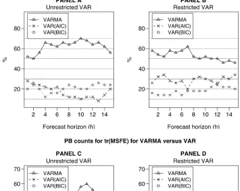
3.1.2 PB Results. The PB counts have been plotted in the
four panels of Figure 1. These plots contain three lines, each one representing a class of models. The points marked on each line depict the percentage of times for which that class of models produces the best forecast for that horizon among all models. For example, consider the 7-step-ahead forecast performance for the VARMA models versus the unrestricted VAR models selected by AIC, that is,VAR(AIC), and those selected by BIC, that is,VAR(BIC). Panel A of Figure 1 shows that the VARMA models outperform both sets of VAR models, as they produce
lower values of|MSFE|approximately 60% of the time. In gen-eral, Panel A of Figure 1 shows that the VARMA models pro-duce the highest PB counts (approximately 60%) for |MSFE| for all h=1- to 15-step-ahead forecast horizons when com-pared to their unrestricted VAR counterparts. A similar con-clusion can be drawn for |MSFE| when we consider as the VARMA counterparts, VAR models whose insignificant lags have been omitted. Panel B of Figure 1 shows that VARMA models produce lower values of |MSFE| than the restricted VAR models, approximately 50 % of the time across all fore-cast horizons. Panels C and D of Figure 1 consider the trace of the MSFE matrix as the accuracy measure. In general, the re-sults are again in favor of VARMA models; however, in these cases there are some forecast horizons for which VAR models outperform VARMA models.
As a general observation for Figure 1 (with the exception of Panel D), VARMA models perform better at least 50% of the time for forecast horizons of more than six or seven steps ahead.
The significance of the 50% value is that if we could somehow choose the best of the VAR models selected by either AIC or BIC, the VARMA models would still “out-forecast” them.
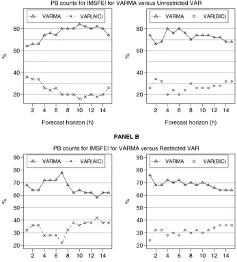
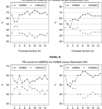
Furthermore, Figures 2 and 3 show a head-to-head compar-ison of the PB counts for the|MSFE|of VARMA models ver-sus VARs, selected by either AIC or BIC. This comparison fur-ther supports the dominance of the VARMA models. Now that the comparison is between VARMA models and one class of VAR models at a time, VARMA models outperform their VAR counterparts for each and every forecast horizon (with the ex-ception ofh=3 for the tr(MSFE), for both unrestricted and restricted VAR models selected by the BIC). The lowest PB count for VARMA models is 44%, for theh=3 forecast hori-zon when compared to the restrictedVAR(AIC), and the highest is 84% percent forh=10 when compared to the unrestricted
VAR(AIC).
The foregoing results show the proportion of times that VARMA models produce a smaller forecast error in compar-ison to VAR models. However, these results do not indicate
Figure 1. PB counts for the|MSFE|and the tr(MSFE)for VARMA models versus unrestricted and restricted VARs selected by the AIC and the BIC.
Figure 2. A head-to-head comparison of PB counts for|MSFE|between VARMA and unrestricted and restricted VAR models selected by either the AIC or the BIC.
whether the differences in forecast errors are statistically sig-nificant. Table 1 summarizes the results of Diebold–Mariano (DM) tests for comparing the tr(MSFE)from VARMA models with unrestricted and restricted VARs selected by AIC and BIC for selected horizons. Note that Figures 2 and 3 show that the |MSFE|favors VARMA models more strongly than the trace, so we have based our significance tests on the less favorable metric. The four numbers in each cell of Table 1 are respec-tively: the percentage of times the DM test statistic was in the lower 5% tail, the lower 25% tail, the upper 25% tail, and the upper 5% tail of a standard Normal distribution. For example, (24,46,20,14)in the cell with the row heading “VAR(AIC)— Unrestricted” and the column heading “1” means that the 1-step-ahead VARMA forecasts were significantly better than the unrestrictedVAR(AIC)forecasts 24% of the time at the 5% level of significance, and 46% of the time at the 25% level of signif-icance. The 1-step-ahead unrestrictedVAR(AIC)forecasts, on the other hand, were significantly better than the VARMA fore-casts 20% of the time at the 25% level of significance, and 14% of the time at the 5% level of significance.
These results show that (1) the PB results are not due to small, insignificant differences between forecasts of different models—there are cases where the VARMA significantly out-performs the VAR and vice versa; (2) the proportion of cases in which VARMA models significantly outperform VAR mod-els is always greater than the reverse; and (3) the number of times that the forecasts of VARMA and VAR models are significantly different from each other decreases with h as expected, because standard errors increase with h. An addi-tional interesting observation is that, even though according to the PB results the performance of VAR(AIC) models be-comes closer to that of VARMA models after the insignif-icant parameters of the VAR have been removed, this table shows that the removal of insignificant parameters must only improveVAR(AIC)forecasts in cases where they are not signif-icantly different from VARMA forecasts, and it actually does not help (and can worsen) the performance of the VAR(AIC) in cases where VARMA models produced significantly better forecasts than VAR(AIC). This shows that the difference be-tween the performance of VARMA and VAR models cannot
Figure 3. A head-to-head comparison of PB counts for tr(MSFE)between VARMA and unrestricted and restricted VAR models selected by either the AIC or the BIC.
be adequately bridged by imposing zero restrictions on VAR models.
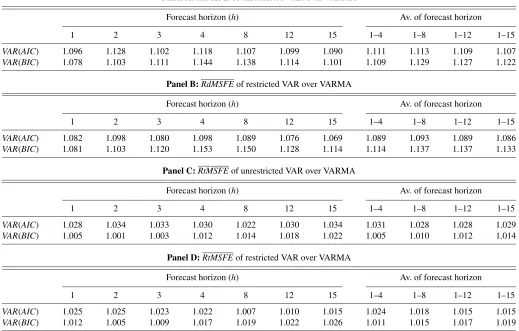
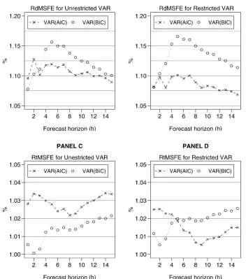
3.1.3 Relative Ratios Results. The results for the relative
ratios are tabulated in Table 2 and plotted in Figure 4. All panels of Table 2 and Figure 4 indicate that all relative ratio measures are consistently greater than 1, for all forecast horizons and for both restricted and unrestricted VARs. A relative ratio greater than 1 shows that VARMA models perform better than VARs
for that forecast horizon. For example, in Panel A forh=4, the determinant of the MSFE matrix for theVAR(AIC)is approx-imately 12% larger than that for the VARMA on average. For the same horizon, the VARMA improvement jumps to approx-imately 14.5% when compared to theVAR(BIC).
The last four columns of each panel of Table 2 show the av-erage relative ratio over several forecast horizons. These also highlight the improvement that VARMA models bring to
out-Table 1. The percentage of times VARMA models produce significantly better multivariate forecasts than VARs and vice versa
Forecast horizon (h)
1 4 8 12 15
VAR(AIC)—Unrestricted 24, 46, 20, 14 16, 38, 10, 0 14, 32, 6, 4 10, 22, 10, 0 10, 22, 8, 0
VAR(BIC)—Unrestricted 24, 50, 22, 12 10, 38, 18, 10 12, 26, 22, 8 12, 18, 16, 4 12, 18, 16, 2
VAR(AIC)—Restricted 34, 54, 26, 12 14, 36, 16, 0 14, 26, 8, 2 12, 22, 10, 0 10, 24, 10, 0
VAR(BIC)—Restricted 32, 54, 22, 14 10, 38, 18, 8 12, 26, 22, 6 10, 20, 20, 6 10, 16, 14, 2
NOTE: The four entries in each cell indicate the percentage of times that the DM test statistic is in the lower 5% tail, lower 25% tail, upper 25% tail, and upper 5% tail of a standard Normal distribution, respectively.
Table 2. Average relative ratios for the determinant and the trace of the MSFE matrices for VAR models selected by AIC and BIC over VARMA
Panel A:RdMSFEof unrestricted VAR over VARMA
Forecast horizon (h) Av. of forecast horizon
1 2 3 4 8 12 15 1–4 1–8 1–12 1–15
VAR(AIC) 1.096 1.128 1.102 1.118 1.107 1.099 1.090 1.111 1.113 1.109 1.107
VAR(BIC) 1.078 1.103 1.111 1.144 1.138 1.114 1.101 1.109 1.129 1.127 1.122
Panel B:RdMSFEof restricted VAR over VARMA
Forecast horizon (h) Av. of forecast horizon
1 2 3 4 8 12 15 1–4 1–8 1–12 1–15
VAR(AIC) 1.082 1.098 1.080 1.098 1.089 1.076 1.069 1.089 1.093 1.089 1.086
VAR(BIC) 1.081 1.103 1.120 1.153 1.150 1.128 1.114 1.114 1.137 1.137 1.133
Panel C:RtMSFEof unrestricted VAR over VARMA
Forecast horizon (h) Av. of forecast horizon
1 2 3 4 8 12 15 1–4 1–8 1–12 1–15
VAR(AIC) 1.028 1.034 1.033 1.030 1.022 1.030 1.034 1.031 1.028 1.028 1.029
VAR(BIC) 1.005 1.001 1.003 1.012 1.014 1.018 1.022 1.005 1.010 1.012 1.014
Panel D:RtMSFEof restricted VAR over VARMA
Forecast horizon (h) Av. of forecast horizon
1 2 3 4 8 12 15 1–4 1–8 1–12 1–15
VAR(AIC) 1.025 1.025 1.023 1.022 1.007 1.010 1.015 1.024 1.018 1.015 1.015
VAR(BIC) 1.012 1.005 1.009 1.017 1.019 1.022 1.026 1.011 1.015 1.017 1.019
of-sample forecasting in comparison to VARs. The last col-umn shows the overall average improvement over all 15 fore-cast horizons. This overall improvement ranges between ap-proximately 1.5%, achieved for the average of the relative ra-tio for the tr(MSFE)for the unrestrictedVAR(BIC)models (see Panel C), and 13.5%, achieved for the average of the relative ratio for the|MSFE|for the restricted VAR(BIC)models (see Panel B).
Whereas the main objective of this forecasting exercise is to compare the forecasting performance of VARMA models with that of VARs, one can also compare the forecast performance of the VAR models selected by the two model selection cri-teria. Figure 4 allows for a head-to-head comparison between the VAR models selected by AIC and those selected by BIC. Panels A and B compare the determinants of the mean squared forecast error matrices for the unrestricted and restricted VARs. Panel A shows that for h≤2, VAR(BIC)perform better, but for allh>2,VAR(AIC)dominate. The performance of the two seems to converge beyondh≥7.
Panel B compares the performance of the restricted VAR models. Recall that the restricted VAR models are VARs with their lag length selected by a model selection criterion and the insignificant individual lags omitted. These results show that the restrictedVAR(AIC)models outperform the restricted
VAR(BIC)models for all forecast horizons. So the conclusion
that we can draw from comparing Panels A and B is that elim-inating insignificant individual lags improves the performance
ofVAR(AIC)models considerably, but it does not improve (in
fact it slightly worsens) the performance of VAR(BIC) els. Panels C and D present the performance of the VAR mod-els based on the tr(MSFE). Again, the message from these figures is thatVAR(AIC)models should be used for forecast-ing only after their insignificant variables have been elimi-nated.
3.2 Method 2: A Four-Variable Quarterly VARMA Model
The analysis in the previous section uses a cross section of 50 trivariate systems and quantifies the relative average perfor-mance of VARMA models versus VARs, without concentrating on any one system in particular. The dataset used (chosen be-cause of its prominence in recent macro-forecasting literature) is of a monthly frequency. However, although monthly data are used in coincident and leading indicator research, they are not used in other areas of applied macroeconomics. We should mention that after a suggestion from one of the referees, we aggregated the monthly datasets to quarterly data and repeated the forecasting exercise of the previous section. The rankings of the models were similar, although the percentage improvements were not as strong as before. In this section, we use quarterly data for four U.S. variables: the GDP growth rate(gt), the 3-month treasury bill rate (rt), the spread between the 10-year government bond yield and the 3-month treasury bill rate(st), and the inflation rate(πt). These four variables have been used
Figure 4. Average relative ratios of the determinant and the trace of the MSFE matrices for VAR models selected by AIC and BIC over VARMA.
extensively in recent years in models of the term structure with observable factors (as in Ang, Piazzesi, and Wei 2006). Fur-thermore, some variations of them are used in New Keynesian dynamic stochastic general equilibrium (DSGE) models (as in contributions in Taylor 1999). In the latter line of research it is common to use some measure of the output gap instead of the output growth rate, and the federal funds rate is used for the short-term interest rate. Later, we add growth rates of real con-sumption expenditure and real investment to this system and repeat the analysis for the six-variable model. The addition of consumption and investment to the list of variables makes the set of variables close to the set used in earlier empirical business cycle papers such as King, Plosser, Stock, and Watson (1991).
All data were downloaded from the Federal Reserve Eco-nomic Database (FRED) in September 2006. The series GDPC96, TB3MS, GS10, CPIAUCSL, PCECC96, and GPDIC96, were chosen for real GDP, 3-month treasury bill rate, 10-year government bond yield, the consumer price in-dex, real personal consumption, and real private investment, respectively. We averaged the interest rates across three months
to convert them to quarterly series, and computed the infla-tion rate as 400 times the difference between the logarithms of the CPI in the last month of the current quarter and the last month of the previous quarter. We use the first difference of the short rate because the graph of the series as well as formal unit root tests indicate that the short rate behaves like an in-tegrated variable of order 1. In the term structure and DSGE articles cited above, the short rate is not differenced, but when examining their empirical results, one can see that the dynamic equation of the short rate has an estimated autoregressive root close to unity, which is often interpreted as evidence of inter-est rate smoothing by the monetary authority. Levin, Wieland, and Williams (1999) argued for using the first difference of the interest rate in monetary policy models because this produces policy rules that are more robust to model uncertainty. Also, in the DSGE literature, a measure of the output gap is used, and at least in articles that use the deviation of log(GDP) from a linear trend, or the difference between log(GDP)and the loga-rithm of the Congressional Budget Office measure of potential output (which is very close to a linear trend), the output gap series is highly persistent, and the estimated dynamic model of
the output gap has a root very close to unity. This means that these estimated models are very similar to a model that uses the output growth rate instead, with one less autoregressive lag. We prefer to work with the output growth rate and the first differ-ence of the short rate here, because the sequdiffer-ence of canonical correlation tests that we perform to develop our VARMA mod-els has asymptotic chi-squared distributions when the series are stationary.
We use quarterly data from 1955 quarter 1 to 1995 quarter 4 (a total of 164 observations) for developing VAR and VARMA models, and we use these estimated models to provide fore-casts from 1996 quarter 1 to 2006 quarter 2 (a total of 42 quar-ters). Two VAR models are developed, one with three lags (cho-sen by the AIC) and the other with two lags (cho(cho-sen by the BIC). Our procedure identifies anSCM(2,0), anSCM(1,1), an SCM(1,0), and anSCM(0,0)for the system. This translates to aVARMA(2,1)model with several rank restrictions in its au-toregressive and moving average parameter matrices. The esti-mated model is
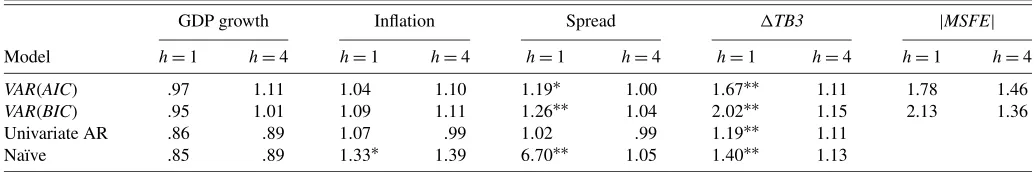
Table 3 summarizes the out-of-sample forecasting perfor-mance results. The two entries in each cell are the ratios of the MSFEs of the one-quarter-ahead and one-year-ahead forecasts of the model in the row heading, relative to VARMA. We do not provide results for longer horizons because no model is signif-icantly better than another for longer horizons. The statistical significance of the difference in MSFEs is shown by a single or double asterisk to denote significant at the 10% and 5% levels of significance, respectively. The last column of this table pro-vides information about the relative determinant of the MSFE matrices for the multivariate models only. The univariate AR models are AR(1) for the GDP growth, AR(3) for inflation and the first difference of the short rate, and AR(2) for the spread. The naïve models forecast that each variable will be constant at its historical mean.
The results in Table 3 show that the VARMA model does not improve the forecasts of the GDP growth or the inflation rate in the last 10 years, although the mean squared forecast errors are not significantly different from each other. This is in line with the recent literature which shows the decline in predictability of output growth and inflation (see D’Agostino, Giannone, and Surico 2006, and references therein). However, the estimated VARMA model provides significantly better 1-step-ahead fore-casts for the term spread and the short rate relative to VAR models. There is a large improvement in the determinant of the MSFE gained by moving from VAR models to VARMA mod-els. It is important to reemphasize that our goal here is to show that with our practical VARMA modeling procedure, there is no compelling reason to use a VAR model as a benchmark multi-variate model in empirical macroeconomic research. Obviously, we do not claim that VARMA models will be more immune to forecast failure than VAR models if there is a structural change toward the end of the estimation sample or during the forecast period. For example, D’Agostino et al. (2006) argued that mul-tivariate models have not been as successful in forecasting GDP growth and inflation after the mid-1980s because the leading in-dicator properties of the spread have changed over this period. If this is the case, VARMA models will not provide any significant improvement for forecasting GDP growth and inflation either. However, for the part of the system that has not suffered from a structural break, such as the short rate and the term spread, the VARMA model is likely to provide significantly better forecasts than the VAR model.
We also performed a similar comparison for a six-variable system, which included growth rates of personal consumption and private investment in addition to the above four variables.
Table 3. Ratio of the MSFE relative to the VARMA model forh=1-step- andh=4-step-ahead forecasts
GDP growth Inflation Spread TB3 |MSFE|
Model h=1 h=4 h=1 h=4 h=1 h=4 h=1 h=4 h=1 h=4
VAR(AIC) .97 1.11 1.04 1.10 1.19∗ 1.00 1.67∗∗ 1.11 1.78 1.46
VAR(BIC) .95 1.01 1.09 1.11 1.26∗∗ 1.04 2.02∗∗ 1.15 2.13 1.36 Univariate AR .86 .89 1.07 .99 1.02 .99 1.19∗∗ 1.11
Naïve .85 .89 1.33∗ 1.39 6.70∗∗ 1.05 1.40∗∗ 1.13
NOTE: The first entry in each cell is the ratio of the MSFE of theh=1-step-ahead forecast of the variable in the column heading, made by the model in the row heading, to the MSFE of the corresponding forecast from the estimated VARMA model. The second entry in each cell is a similar ratio corresponding to theh=4-step ahead forecasts. If a ratio is significantly different from 1 at the 5% level of significance, it is superscripted by∗∗, and if it is significant at the 10% level of significance, it is superscripted by∗.
The motivation behind this is the empirical real business cycle model as in King et al. (1991). The determinant of the MSFE matrix of the VARMA model for this system is less than two-thirds of that of the VAR model, for both 1-step and 4-step ahead forecasts. We do not provide detailed results here, but they are available upon request.
3.3 Why Do VARMA Models Produce Better
Forecasts Than VARs?
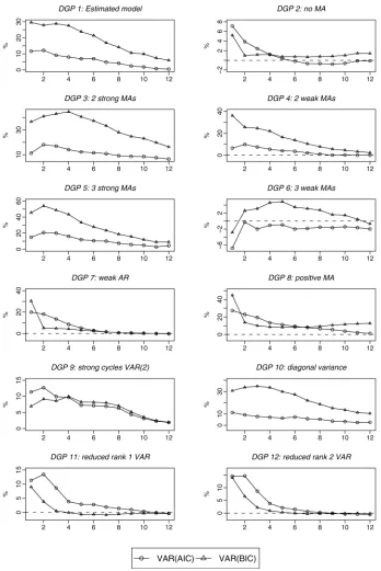
A natural question that arises from the foregoing exercises is, why do VARMA models perform better than VARs for mul-tivariate forecasting? The intuitive answer to this is that there must be significant finite vector moving average (VMA) com-ponents in systems of macroeconomic variables that cannot be adequately approximated by short-order VARs. However, our scalar component methodology discovers cross-equation restrictions at the same time as identifying the structure of the VARMA model. Is the improved forecasting performance due to our allowance for moving average components, or mostly as a result of our consideration of cross-equation restrictions? We investigate this by the following simulation study. We use the estimated four-variableVARMA(2,1)model from the previous section as the benchmark data generating process (DGP), as-suming that it has multivariate Normal errors. In each iteration, we generate 406 observations. We discard the first 200 obser-vations, use the next 164 to estimate VARMA and VAR mod-els, and use the remaining 42 observations for an out-of-sample forecast evaluation. We repeat this exercise 100 times and av-erage the determinants of the MSFE matrices of VARMA and VAR models to obtain estimates of their expected values. We then compute the difference between the expected|MSFE|of VARMA and VAR models as a percentage of the latter. The re-sults for 1- to 12-step-ahead forecasts are plotted in the top left panel of Figure 5, titled “DGP1: Estimated model.” We then vary specific features of the DGP, one at a time, and repeat the exercise for each case. The variations that we consider are listed in Table 4.
Figure 5 summarizes the results. Each panel plots the per-centage improvement in the |MSFE| of VARMA versus the VAR chosen by AIC and the VAR chosen by BIC for 1- to 12-step-ahead forecasts. Care should be taken when compar-ing these, as the scale of the vertical axis is not the same for all plots.DGP2 shows the importance of moving average terms. With no moving average terms, the only advantage the SCM modeling strategy has over VARs is the possibility of discov-ering reduced rank in the autoregressive parameter matrices, which only improves the determinant of the MSFE by 8% at most. This shows that the inadequacy of the VARs, in partic-ular those selected by BIC, is caused by the MA components in the DGP. Increasing the number of strong MA components, as inDGP3andDGP5, exacerbates the advantage of VARMA models over VARs. However,DGP6shows that if there are sev-eral weak moving averages in the DGP, there is no advantage of considering VARMA models. We think that the uncertainty in the estimation of many small coefficients based on a sample of 164 observations causes the VARMA model to perform worse than the VAR in this case.
DGP7 shows that with less persistence in the data, the ad-vantage of allowing for VARMA models will be restricted to
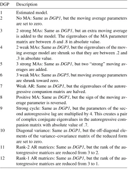
Table 4. A short description of the DGPs used in the simulation study
DGP Description
1 Estimated model.
2 No MA: Same asDGP1, but the moving average parameters are set to zero.
3 2 strong MAs: Same asDGP1, but an extra moving average is added to the model. The eigenvalues of the MA parameter matrix are between .6 and .8 in absolute value.
4 2 weak MAs: Same asDGP3, but the eigenvalues of the mov-ing average model are shrunk so that they are between .2 and .3 in absolute value.
5 3 strong MAs: Same asDGP1, but two “strong” moving av-erages are added.
6 3 weak MAs: Same asDGP5, but moving average parameters are shrunk toward zero.
7 Weak AR: Same asDGP1, but the eigenvalues of the autore-gressive companion matrix are halved.
8 Positive MA: Same asDGP1, but the sign of the moving av-erage parameter is reversed.
9 Strong cycle: Same asDGP1, but the parameters of the sec-ond autoregressive lag are multiplied by 4. This creates a pair of complex conjugate eigenvalues in the autoregressive com-panion matrix with absolute value of .7.
10 Diagonal variance: Same asDGP1, but the off-diagonal ele-ments of the variance–covariance matrix of the reduced form are set to zero.
11 Rank-2 AR matrices: Same asDGP1, but the rank of the au-toregressive matrices are reduced from 3 to 2.
12 Rank-1 AR matrices: Same asDGP1, but the rank of the au-toregressive matrices are reduced from 3 to 1.
short-term forecasts, which is quite plausible.DGP8 reverses the signs of the moving average parameters. Although the ad-vantage of VARMA models over short horizons stays the same as the benchmark, there is less persistence in this advantage over longer horizons, especially relative to the VARs selected by BIC. This shows that when the roots of the autoregressive and the moving average characteristic polynomials are of the same sign (as in the benchmark DGP), BIC is more likely to wrongly assume that these roots are of the same magnitude and to choose a severely underparameterized VAR model, which produces very inaccurate forecasts. This is confirmed by the large number ofVAR(1)’s chosen by BIC in the baseline case relative toDGP8, as is reported in Table 5. InDGP9, the para-meters of the second autoregressive lag are larger in absolute value than the baseline DGP, and this causes stronger cycli-cal dynamics in the variables. Quite plausibly, this improves the performance of VAR models, in particularVAR(BIC). Set-ting the off-diagonal elements of the error covariance matrix in
DGP10to zero seems to make little difference to the relative
performance of different models. Finally, changing the autore-gressive parameters of the baseline DGP to introduce a more severe rank deficiency in the system makes little difference to the performance of the VAR models chosen by AIC, but it im-proves the performance of those selected by BIC. This is per-haps because when the autoregressive parameter matrices are sparse, aVAR(1)is a better approximation of the DGP than a longer VAR chosen by AIC.
The foregoing exercise suggests that the bulk of the dif-ference between the forecasting performance of VARMA and
Figure 5. Percentage improvement for|MSFE|for VARMA versusVAR(AIC)andVAR(BIC).
VAR models is due to significant moving average terms in the data generating process. Although this conclusion is quite in-tuitive, one must be careful that different perturbations of the baseline DGP are not “similar.” For example, the changes in the baseline DGP that lead toDGP2may be quite a larger pertur-bation than those that lead toDGP7according to any measure of distance between stochastic processes.
4. CONCLUSION
The message of this article is that we can obtain better fore-casts for macroeconomic variables if we consider VARMA
models rather than restricting ourselves to VAR models. With recent methodological advances in the identification and esti-mation of VARMA models, and with the improvement in com-puting power and econometrics software, there is no compelling reason to restrict the class of models to VARs only. Our empir-ical results show that VARMA models developed by a scalar component methodology outperform VAR models in forecast-ing macroeconomic variables. Are these favorable results spe-cific to the VARMA models developed by the scalar compo-nent methodology that we adopt in this paper? The answer is no. Athanasopoulos (2005) showed that the same conclusion emerges when one uses an “Echelon form” approach
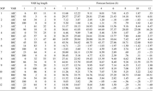
Table 5. Percentage improvement for the|MSFE|for VARMA versus VAR for the Monte Carlo simulation study
VAR lag length Forecast horizon (h)
DGP VAR 1 2 3 4 1 2 3 4 6 8 10 12
1 AIC 6 83 11 0 11.68 12.22 9.11 8.01 7.01 4.15 1.87 .53 BIC 95 5 0 0 29.57 27.87 28.81 27.60 21.43 14.18 9.93 6.01 2 AIC 64 34 2 0 7.12 3.87 2.45 1.20 −.18 −.69 −.63 −.10 BIC 100 0 0 0 5.20 1.00 1.16 1.21 .75 .79 1.02 1.42 3 AIC 1 61 32 6 11.17 18.13 16.93 14.06 11.56 9.16 8.44 6.47 BIC 90 10 0 0 36.61 41.05 43.03 44.69 37.37 28.05 23.08 16.28 4 AIC 0 75 25 0 6.46 9.89 7.48 5.46 3.59 1.07 .29 .03 BIC 43 57 0 0 36.25 25.60 24.61 22.04 13.77 7.80 4.60 2.37 5 AIC 0 13 47 40 14.95 20.84 20.00 16.19 10.64 7.42 4.87 4.46 BIC 45 55 0 0 45.54 54.02 48.75 43.37 27.86 18.71 12.00 9.03 6 AIC 14 83 3 0 −6.71 −.23 −1.97 −1.03 −1.97 −1.50 −1.42 −1.97 BIC 100 0 0 0 −2.83 2.60 3.11 4.59 3.49 2.74 1.47 −.66 7 AIC 23 64 9 4 20.00 18.11 13.59 8.59 2.89 .69 .33 −.23 BIC 100 0 0 0 30.45 5.18 4.77 4.33 2.39 .76 .11 −.01 8 AIC 0 32 53 15 27.41 22.92 19.43 13.39 9.40 6.62 3.90 1.35 BIC 66 34 0 0 44.81 13.70 10.05 8.67 8.40 9.28 11.55 12.75 9 AIC 0 75 20 5 11.37 12.74 9.95 9.67 7.14 6.35 3.12 1.90 BIC 0 100 0 0 6.93 9.20 8.62 9.97 8.19 7.08 3.57 1.98 10 AIC 6 86 8 0 11.26 9.21 7.76 7.07 7.30 5.25 3.22 2.62 BIC 98 2 0 0 30.76 33.75 34.76 33.62 27.29 18.73 13.60 10.51 11 AIC 34 54 10 2 11.32 13.46 8.66 3.84 2.82 1.45 .41 −.30 BIC 100 0 0 0 9.03 3.82 .56 −.05 −.64 −.56 −.28 −.37 12 AIC 23 64 9 4 14.58 14.67 8.64 3.80 1.50 .29 −.34 −.60 BIC 100 0 0 0 13.96 6.61 2.21 .94 −.05 −.22 −.18 −.14
NOTE: Column 1, labelled “DGP,” indicates the data generating process from which we have simulated. Column 2, labelled “VAR,” indicates the model selection criterion used for selecting VAR models. Each entry in the columns under the heading “VAR lag length” shows the percentage of times that the model selection criterion selected a VAR of the specified length. Each entry in the columns under the heading “Forecast horizon (h)” specifies the percentage improvement for the|MSFE|that VARMA models achieve relative to VARs.
nan and Deistler 1988; Lütkepohl and Poskitt 1996) to de-velop VARMA models. Our analysis in this article suggests that the existence of strong vector moving average components that cannot be well-approximated by finite-order vector autoregres-sions is the most likely reason for the superior performance of VARMA models relative to VARs for macroeconomic forecast-ing.
ACKNOWLEDGMENTS
We acknowledge valuable comments and suggestions from Heather Anderson, Don Poskitt, James Nason, Rob Hyndman, Torben Andersen (editor), an associate editor, two anonymous referees, seminar participants at Monash University, Queens-land University of Technology, the 2004 Australasian Meeting of the Econometric Society, and the 2004 International Sympo-sium on Forecasting. We are also thankful to Cathy Morgan and Despina Iliopoulos for copyediting assistance. George Athana-sopoulos acknowledges the financial support from Tourism Australia and the Sustainable Tourism Cooperative Research Centre. Farshid Vahid acknowledges financial support from Australian Research Council grant DP0343811.
APPENDIX: DATA SUMMARY
This appendix lists the time series that are used in this arti-cle. The series have been directly downloaded from Mark Wat-son’s web page (http://www.wws.princeton.edu/mwatson/). The names (mnemonics) given to each series and the brief descrip-tion following each series name have been reproduced from
Watson (2003). The superscript index on the series name is the transformation code which corresponds to (1) the level of the series, (2) the first difference (yt=yt−yt−1), and (3) the first difference of the logarithm, that is, series transformed to growth rates(100∗lnyt). The following abbreviations also appear in the brief data descriptions: SA=seasonally adjusted; SAAR=seasonally adjusted at an annual rate; NSA=not sea-sonally adjusted.
(i)Output and income
1. IP3 Industrial production: total index (1992=100, SA)
2. IPP3 Industrial production: products, total (1992=100, SA)
3. IPF3 Industrial production: final products (1992=100, SA)
4. IPC3 Industrial production: consumer goods (1992=100, SA)
5. IPUT3 Industrial production: utilities (1992=100, SA)
6. PMP1 NAPM production index (percent) 7. GMPYQ3 Personal income (chained) (series #52)
(Bil 92$, SAAR)
(ii)Employment and hours
8. LHUR1 Unemployment rate: all workers, 16 years and over (%, SA)
9. LPHRM1 Avg. weekly hrs. of production wkrs.: mfg., manufacturing (SA)
10. LPMOSA1 Avg. weekly hrs. of production wkrs.: mfg., overtime hrs. (SA)
11. PMEMP1 NAPM employment index (percent)
(iii)Consumption, manufacturing and retail sales, and housing
12. MSMTQ3 Manufacturing and trade: total (mil of chained $1992 SA)
13. MSMQ3 Manufacturing and trade: manufactur-ing, total (mil of chained $1992 SA) 14. MSDQ3 Manufacturing and trade:
manufactur-ing, durable goods (mil of chained $1992 SA)
15. MSNQ3 Manufacturing and trade: manufactur-ing, nondurable goods (mil of chained $1992 SA)
16. WTQ3 Merchant wholesalers: total (mil of chained $1992 SA)
17. WTDQ3 Merchant wholesalers: durable goods total (mil of chained $1992 SA) 18. WTNQ3 Merchant wholesalers: nondurable
goods total (mil of chained $1992 SA) 19. RTQ3 Retail trade: total (mil of chained $1992
SA)
20. RTNQ3 Retail trade: nondurable goods (mil of chained $1992 SA)
21. CMCQ3 Personal consumption expend—total (bil of chained $1992 SAAR)
(iv)Real inventories and inventory-sales ratios
22. IVMFGQ3 Inventories, business, manufacturing (mil of chained $1992 SA)
23. IVMFDQ3 Inventories, business durables (mil of chained $1992 SA)
24. IVMFNQ3 Inventories, business nondurables (mil of chained $1992 SA)
25. IVSRQ2 Ratio for manufacturing and trade: inventory/sales (chained $1992 SA) 26. IVSRMQ2 Ratio for manufacturing and trade:
man-ufacturing inventory/sales ($1987 SA) 27. IVSRWQ2 Ratio for manufacturing and trade:
wholesaler; inventory/sales ($1987 SA) 28. IVSRRQ2 Ratio for manufacturing and trade: retail
trade; inventory/sales ($1987 SA) 29. MOCMQ3 New orders (net)—consumer goods and
materials ($1992 BCI)
30. MDOQ3 New orders, durable goods industries ($1992 BCI)
(v)Prices and wages
31. PMCP1 NAPM commodity prices index (per-cent)
(vi)Money and credit quantity aggregates
32. FM2DQ3 Money supply—M2 in ($1992 BCI) 33. FCLNQ3 Commercial and industrial loans
out-standing in ($1992 BCI)
(vii)Interest rates
34. FYGM32 Interest rate: US treasury bills, sec mkt, 3-MO (% p.a. NSA)
35. FYGM62 Interest rate: US treasury bills, sec mkt, 6-MO (% p.a. NSA)
36. FYGT12 Interest rate: US treasury const maturi-ties, 1-YR (% p.a. NSA)
37. FYGT102 Interest rate: US treasury const maturi-ties, 10-YR (% p.a. NSA)
38. TBSPR1 Term spread FYGT10–FYGT1
(viii)Exchange rates, stock prices and volume
39. FSNCOM3 NYSE common stock prices index: composite (12/31/65=50)
40. FSPCOM3 S&P’s common stock prices index: composite (1941–43=10)
[Received January 2006. Revised March 2007.]
REFERENCES
Ang, A., Piazzesi, M., and Wei, M. (2006), “What Does the Yield Curve Tell Us About GDP Growth?”Journal of Econometrics, 131, 359–403. Athanasopoulos, G. (2005), “Essays on Alternative Methods of Identification
and Estimation of Vector Autoregressive Moving Average Models,” unpub-lished doctoral dissertation, Monash University, Dept. of Econometrics and Business Statistics.
Athanasopoulos, G., and Vahid, F. (2006), “A Complete VARMA Modelling Methodology Based on Scalar Components,” working paper, Monash Uni-versity, Dept. of Econometrics and Business Statistics.
Clark, T. E., and McCracken, M. W. (2001), “Tests of Equal Forecast Accu-racy and Encompassing for Nested Models,”Journal of Econometrics, 105, 85–110.
Clements, M. P., and Hendry, D. F. (1993), “On the Limitations of Comparing Mean Squared Forecast Errors” (with discussions),Journal of Forecasting, 12, 617–637.
Corradi, V., and Swanson, N. (2002), “A Consistent Test for out of Sample Nonlinear Predictive Ability,”Journal of Econometrics, 110, 353–381.
(2007), “Nonparametric Bootstrap Procedures for Predictive Inference Based on Recursive Estimation Schemes,”International Economic Review, 48, 67–109.
D’Agostino, A., Giannone, D., and Surico, P. (2006), “(Un)predictability and Macroeconomic Stability,” Working Paper 605, European Central Bank. Diebold, F. X., and Mariano, R. S. (1995), “Comparing Predictive Accuracy,”
Journal of Business & Economic Statistics, 13, 253–263.
Durbin, J. (1963, 1988), “Maximum Likelihood Estimation of the Parameters of a System of Simultaneous Regression Equations,”Econometric Theory, 4, 159–170.
Giacomini, R., and White, H. (2006), “Tests of Conditional Predictive Ability,” Econometrica, 74, 1545–1578.
Hannan, E. J. (1969), “The Identification of Vector Mixed Autoregressive-Moving Average Systems,”Biometrika, 56, 223–225.
Hannan, E. J., and Deistler, M. (1988),The Statistical Theory of Linear Systems, New York: Wiley.
Hannan, E. J., and Rissanen, J. (1982), “Recursive Estimation of Autoregres-sive-Moving Average Order,”Biometrika, 69, 81–94.
Hillmer, S. C., and Tiao, G. C. (1979), “Likelihood Function of Stationary Mul-tiple Autoregressive Moving Average Models,”Journal of the American Sta-tistical Association, 74, 652–660.
King, R. G., Plosser, C. I., Stock, J., and Watson, M. W. (1991), “Stochas-tic Trends and Economic Fluctuations,”American Economic Review, 81, 819–840.
Levin, A. T., Wieland, V., and Williams, J. C. (1999), “Robustness of Simple Monetary Policy Rules Under Model Uncertainty,” inMonetary Policy Rules, ed. J. B. Taylor, Chicago: University of Chicago Press, pp. 622–645. Lütkepohl, H. (1993),Introduction to Multiple Time Series Analysis(2nd ed.),
Berlin–Heidelberg: Springer-Verlag.
Lütkepohl, H., and Poskitt, D. (1996), “Specification of Echelon-Form VARMA Models,”Journal of Business & Economic Statistics, 14, 69–79.
Makridakis, S., and Hibon, M. (2000), “The M3-Competition: Results, Conclu-sions and Implications,”International Journal of Forecasting, 16, 451–476. Poskitt, D. S. (1992), “Identification of Echelon Canonical Forms for
Vec-tor Linear Processes Using Least Squares,”The Annals of Statistics, 20, 195–215.
Quenouille, M. H. (1957), The Analysis of Multiple Time Series, London: Charles Griffin and Company.
Reinsel, G. (1997),Elements of Multivariate Time Series(2nd ed.), New York: Springer-Verlag.
Sims, C. A. (1980), “Macroeconomics and Reality,”Econometrica, 48, 1–48. Stock, J., and Watson, M. W. (1999), “A Comparison of Linear and Nonlinear
Univariate Models for Forecasting Macroeconomic Time Series,” in Coin-tegration, Causality and Forecasting, eds. R. F. Engle and H. White, New York: Oxford University Press, pp. 1–44.
Sullivan, R., Timmermann, A., and White, H. (1999), “Data-Snooping, Tech-nical Trading Rule Performance, and the Bootstrap,”Journal of Finance, 54, 1647–1692.
Taylor, J. B. (ed.) (1999), “Monetary Policy Rules,” inMonetary Policy Rules, Chicago: University of Chicago Press, pp. 319–341.
Tiao, G., and Tsay, R. (1989), “Model Specification in Multivariate Time Se-ries” (with discussions),Journal of the Royal Statistical Society, Ser. B, 51, 157–213.
Tiao, G. C. (2001), “Vector ARMA,” inA Course in Time Series Analysis, eds. D. Peña, G. C. Tiao, and R. S. Tsay, New York: John Wiley and Sons, pp. 365–407.
Tiao, G. C., and Box, G. E. P. (1981), “Modelling Multiple Time Series With Applications,”Journal of the American Statistical Association, 76, 802–816.
Tsay, R. S. (1991), “Two Canonical Forms for Vector ARMA Processes,” Sta-tistica Sinica, 1, 247–269.
Tunnicliffe-Wilson, G. (1973), “The Estimation of Parameters in Multivariate Time Series Models,”Journal of the Royal Statistical Society, Ser. B, 35, 76–85.
Vahid, F., and Issler, J. (2002), “The Importance of Common Cyclical Fea-tures in VAR Analysis: A Monte-Carlo Study,”Journal of Econometrics, 109, 341–363.
Watson, M. W. (2003), “Macroeconomic Forecasting Using Many Predictors,” in Advances in Economics and Econometrics, Theory and Applications, Vol. III, eds. M. Dewatripont, L. Hansen, and S. Turnovsky, Cambridge: Cambridge University Press, pp. 87–115.
West, K. D. (1996), “Asymptotic Inference About Predictive Ability,” Econo-metrica, 64, 1067–1084.
Wold, H. (1938),A Study in the Analysis of Stationary Time Series, Stockholm: Almqvist and Wiksell.
Zellner, A. (1963), “Estimators for Seemingly Unrelated Regression Equations: Some Exact Finite Sample Results,”Journal of the American Statistical As-sociation, 58, 977–992.