Full Terms & Conditions of access and use can be found at
http://www.tandfonline.com/action/journalInformation?journalCode=ubes20
Download by: [Universitas Maritim Raja Ali Haji] Date: 12 January 2016, At: 22:59
Journal of Business & Economic Statistics
ISSN: 0735-0015 (Print) 1537-2707 (Online) Journal homepage: http://www.tandfonline.com/loi/ubes20
Estimating and Combining National Income
Distributions Using Limited Data
Duangkamon Chotikapanich, William E Griffiths & D. S. Prasada Rao
To cite this article: Duangkamon Chotikapanich, William E Griffiths & D. S. Prasada Rao (2007)
Estimating and Combining National Income Distributions Using Limited Data, Journal of Business & Economic Statistics, 25:1, 97-109, DOI: 10.1198/073500106000000224
To link to this article: http://dx.doi.org/10.1198/073500106000000224
Published online: 01 Jan 2012.
Submit your article to this journal
Article views: 107
View related articles
Estimating and Combining National Income
Distributions Using Limited Data
Duangkamon C
HOTIKAPANICHDepartment of Econometrics and Business Statistics, Monash University, Melbourne, Australia (Duangkamon.Chotikapanich@buseco.monash.edu.au)
William E. G
RIFFITHSDepartment of Economics, University of Melbourne, Melbourne, Australia
D. S. P
RASADAR
AODepartment of Economics, University of Queensland, Brisbane, Australia
A major problem encountered in studies of income inequality at regional and global levels is estimating income distributions from data that are in summary form. In this article we estimate national and regional income distributions within a general framework that relaxes the assumption of constant income within groups. We propose a technique to estimate the parameters of a beta-2 distribution using grouped data. We model regional income distribution using a mixture of country-specific distributions and examine its properties. We use the techniques to analyze national and regional inequality trends for eight East Asian countries and two benchmark years, 1988 and 1993.
KEY WORDS: Beta-2 distribution; Gini coefficient.
1. INTRODUCTION
In the current climate of increasing globalization and a push for free trade among nations, there is concern that increasing globalization may lead to increasing inequality, and that in-creasing global inequality may mean the unsustainability of the current international order. Central to the ongoing debate about globalization are the problem of measuring the extent of economic inequality and the need to be able to meaningfully compare inequality across countries, regions, and time peri-ods. Unless we can measure well and compare well, we can-not easily evaluate whether various policy initiatives that move toward greater globalization, or have other related impacts, are increasing or reducing inequality. The current literature on the subject (Chotikapanich, Valenzuela, and Prasada Rao 1997; Bourguignon and Morrisson 1999; Dowrick and Akmal 2001; Milanovic 2002a, b; Sala-i-Martin 2002a, b; Bhalla 2002; Quah 2002) demonstrates varying results in terms of the levels and trends of inequality. In general, results appear to be sensitive to the measures of income, inequality data, and the methodology used in studying regional and global inequality.
A crucial component of the estimation of global inequality is the intracountry inequality measurement for all countries in-cluded in the study. Much of the earlier work in the area of global inequality, due to Theil (1989), was focused on inter-country inequality and ignored inequality within each inter-country. In recent years it has become common to use global inequal-ity measures that incorporate measures of inequalinequal-ity within each country. Typically, when using data for cross-country and regional comparisons, limited information is available on the level of inequality within each country. Most available data are in the form of either some measure of inequality, such as the Gini coefficient, or income shares of quintile or decile groups. Chotikapanich et al. (1997) used information on Gini coefficients—their work was based on the assumption that the income distribution in each country follows a lognormal distri-bution. More recent work by Milanovic (2002a), Sala-i-Martin
(2002a, b), and Dowrick and Akmal (2001) makes use of in-come share data for deciles and quintiles of each country’s pop-ulation, with Deininger and Squire (1996) being the primary source of data. An important consideration when using decile or quintile share data is the treatment of inequality within each population (e.g., decile) group. In some studies there is an im-plied assumption that there is no within-group inequality and each individual in an income group receives the same income. In other studies kernel smoothing has been used. Sala-i-Martin (2002a, b) used kernel smoothing methods to derive the distri-bution of income within each country, and Milanovic (2002a) and Sala-i-Martin (2002a, b) used kernel smoothing techniques to derive the global distribution of income. This approach is also used in the more recent work of Dowrick, Eckland, and Freyens (2004), in which global poverty estimates are computed from national and global income distributions derived using kernel smoothing.
In a recent critique of the work of Sala-i-Martin (2002b), Milanovic (2002b) demonstrated the sensitivity of the estimates of levels of and trends in global income distribution to the methodology used. He demonstrated, using a simulated exam-ple, that use of kernel smoothing to derive country-specific in-come distributions from quintile share data can produce strange outcomes. He also provided evidence that global income dis-tributions and measures appear to be sensitive to the choice of methodology used to analyze intracountry inequality when us-ing limited data. An alternative assumption of equal distribu-tion of income within each income quintile or decile is equally untenable when income distributions are known to be highly skewed.
© 2007 American Statistical Association Journal of Business & Economic Statistics January 2007, Vol. 25, No. 1 DOI 10.1198/073500106000000224
97
There is a general recognition that estimates of global income inequality and its underlying distribution would be vastly im-proved if country-specific income distributions could be mod-eled adequately. The main constraint on this endeavor is the limited nature of data available. We are typically faced with a problem of using decile group data, with 10 pieces of infor-mation, to model more general and complex distributions than the lognormal distribution used by Chotikapanich et al. (1997). The main objective of this article is to describe a method for estimating the parameters of a relatively flexible form of in-come distribution using a limited amount of data. The success and effectiveness of the proposed methodology is assessed by applying goodness-of-fit criteria to the fitted income distribu-tion. We establish the feasibility and usefulness of estimating a beta-2 distribution (McDonald 1984), a distribution known to be flexible in modeling various income distributions and known to fit income distributions well.
Given a parametric description of the distribution of income in each country, we show how global and regional distribu-tions can be studied in detail by considering them as a mix-ture of the country-specific distributions with population shares as weights. Methods for measuring regional inequality from the mixture distribution are also outlined. The empirical example in this article should be considered illustrative in nature, designed to demonstrate the feasibility of the proposed method. The data used are those compiled and used by Milanovic (2002a); they comprise mean income for each of a number of population groups ordered from poorest to richest. The proposed method-ology is illustrated using data from eight selected East Asian countries: Hong Kong, Japan, Malaysia, Philippines, Singa-pore, Korea, Taiwan, and Thailand. We fit a beta-2 distribution for each country and compute a regional income distribution as a weighted average of the country-specific income distributions. This procedure is applied to data for two years, 1988 and 1993. The adequacy of the beta distribution is assessed through a com-parison of predicted and actual income shares and Gini coeffi-cients.
An outline of the article is as follows. In Section 2 we de-scribe the basic data and their sources. We discuss the method-ology used to estimate the parameters of the income distribution of a given country, assuming that it follows a beta-2 distribution, in Section 3. We also outline an analytical framework to study regional inequality as a mixture of the country-specific distribu-tions. In Section 4 we present empirical results from application of the methodology to the eight selected countries. The results show that inequality within countries increased over the period 1988–1993, but inequality within the region comprising those countries did not change. We provide some concluding remarks and possible areas for further research in Section 5.
2. DESCRIPTION OF DATA AND SOURCES
Compilation of data on income distributions from a large set of countries spanning a long period is a major research problem. Fortunately, the World Bank has long been a major provider of income-distribution data for the purpose of cross-country re-search. Recent work by Milanovic (2002a) is based on a set of cross-country data that he compiled for the World Bank. We use the same set of data. For each country, class mean incomes
(or expenditures) are given in local currency for a number of income classes, ranging from 10 to 20. For each income class, the population share is known. Data are available for more than 100 countries for 1988 and 1993. The data on our selected East Asian countries come from this source with the exception of Singapore in 1988. Singapore was not included in the dataset for this year, so we use data from the International Labor Office (1995) as an alternative source for this case. This dataset is dif-ferent from those obtained from Milanovic (2002a), consisting of decile expenditure shares.
Ideally, distribution data should refer to either income or ex-penditure of persons or households. In the current dataset, there is a mix of per capita income and per capita expenditure. Most data are for the distribution of incomes; the exceptions where the distribution of expenditures is used are Singapore in 1988, Philippines in both 1998 and 1993, and Thailand in 1993. These differences could influence the estimates of the parameters of the respective “income” distributions.
To derive the income distribution for the region as a whole, nominal per capita income for each country must be adjusted for differences in prices across countries, and for the pur-pose of temporal welfare comparisons, further adjustments are needed for movement in prices over time. To describe how such adjustments are made, consider first the original data from each country in one particular year. Letxi¯ represent the class mean income (or expenditure) in local currency and ci
rep-resent the population share for the ith income class. Based on these data, we calculate the income share for each in-come class asgi= ¯xici/x¯jcj. To adjust for purchasing power
parity (over countries and time), we obtain data on real per capita income from the latest version of the Penn World Ta-bles, PWT 6.1, which have data on real per capita incomes for more than 150 countries spanning a 50-year period. PWT 6.1 (http://pwt.econ.upenn.edu/php_site/pwt_index.php) also pro-vide data on the population size of each of the countries. For each country and for a given year, lety¯ be the real per capita income adjusted for differences in prices across countries and over time and letSbe the size of the population. For each come group in a country the real class mean income for in-come class i, y¯i, is derived as total income in the ith group, giyS¯ , divided by total population in the ith group,ciS, that is, ¯
yi=giy¯/ci. Values forxi¯, ci, ¯y, and S used in this article are given in Appendix A, Tables A.1 and A.2. Data on ci andx¯i
are drawn from an article by Milanovic (2002a); these are used only in determining income shares in each of the decile groups. Data forSandy¯are from PWT6.1. The PWT income data are used to calculate average income,y¯i, for the ith decile group.
The valuesy¯iandciare those used in the later analysis.
To provide an accurate assessment of the levels and trends in regional inequality, leading to a basis for informed debate on the effect of globalization on inequality, our study should ide-ally cover a period of at least the last two decades. The current empirical application of the methodology has been restricted to two benchmark years, 1988 and 1993; these are the two years of focus in the study of Milanovic (2002a). At the time that this article was prepared, it was not possible to obtain income distribution data for the most recent years.
3. ESTIMATION OF COUNTRY–SPECIFIC INCOME DISTRIBUTIONS
A large number of probability density functions (pdf’s) have been suggested in the literature for modeling income distribu-tions (see, e.g., McDonald and Ransom 1979; McDonald 1984; McDonald and Xu 1995; Creedy and Martin 1997; Bandourian, McDonald, and Turley 2002; Kleiber and Kotz 2003). The one that we have chosen for our analysis is a member of the McDonald family of distributions (see McDonald and Xu 1995) known as the beta-2 distribution. The beta-2 distribution has been extensively used in modeling income distribution data; it has a number of convenient analytical properties, and, as we discuss later, it provides a very good fit to the observed data. Slottje (1984, 1987) showed how a multivariate beta-2 distrib-ution can be used to model the joint distribdistrib-ution of component sources of income that define the total income of a population unit, as well as the distribution of expenditures on various com-modity groups that aggregate to total consumption expenditure. He demonstrated that the marginal distribution of each income and expenditure component follows beta-2 distributions. In ad-dition, the beta-2 distribution has the desirable property that the marginal distributions of the total income and expenditure ag-gregates follow beta-2 distributions. As a corollary, the Gini co-efficients for the aggregate and their components have the same functional forms but with different parameter values.
Our estimation problem is to estimate the parameters of uni-variate beta-2 distributions for each of the countries in our study when only limited grouped data are available. We then proceed to model regional income as a mixture of the estimated country-specific beta distributions. A similar work by Chotikapanich et al. (1997) used a lognormal distribution to model the income distributions for each country. Although the lognormal distri-bution is relatively easy to estimate from information on the Gini coefficients and mean income for each country, it is known to be restrictive in that it implies symmetric and nonintersect-ing Lorenz curves. The beta-2 distribution is a more flexible distribution; given that it depends on three rather than two un-known parameters, it has the potential to provide a better fit to the data. In Section 3.1 we describe the beta-2 distribution and its characteristics. In Section 3.2 we outline a method for esti-mating its parameters and the class limits of the grouped data. To assess whether estimation of the beta distribution provides an improvement over the more straightforward lognormal dis-tribution, in Appendix B we describe how a similar exercise can be carried out using a lognormal distribution and compare the goodness of fits. The results support the use of the beta-2 distri-bution. We present methods for combining the country-specific income distributions and exploring the characteristics of the re-sulting regional income distribution in Section 3.3.
3.1 The Beta-2 Income Distribution
The beta-2 distribution with parametersb,p, andq that we wish to estimate has pdf
f(y)= y mean to exist,q>1 is required.
The corresponding cumulative distribution function (cdf ) is given by
The functionBt(p,q)is the cdf for the normalized beta distrib-ution defined on the(0,1)interval. It is a convenient represen-tation because it is commonly included as a readily computed function in statistical software. IfT is a standard beta random variable defined on the interval(0,1), then the relationship be-tweenTandYis
T= Y
b+Y, Y= bT
1−T.
The mean, mode, and variance ofY are given by
µ= bp
The estimation procedure that we describe in Section 3.2 re-quires starting values forb,p, andq. It is often easier to suggest reasonable starting values forµ,m, andσ2. In this case corre-sponding values forb,p, andqcan be found from
For future reference, we note that the Gini coefficient is given by
G=2B(2p,2q−1)
pB2(p,q) . (5) We use the Gini coefficient to illustrate how country and re-gional inequalities can be calculated within the framework of our analysis. Other inequality measures could be considered. Decomposition of inequality was not the focus of our study, but for studies where it is a concern, using entropy measures, as ad-vocated by Theil (1989), has the advantage of decomposability.
3.2 Estimating Parameters of the Beta-2 Distribution
Suppose that we have N income classes, (a0,a1), (a1,a2),
. . . , (aN−1,aN), witha0=0 andaN= ∞. Let the mean class
incomes for each of theN classes be given by¯y1,¯y2, . . . ,yN¯ , and let the population proportions for each class be given by
c1,c2, . . . ,cN. Given available data on they¯iand theci, but not
theai, our problem is to estimate the parameters of a beta-2
dis-tribution, along with the unknown class limitsa1,a2, . . . ,aN−1. One approach is to fit a beta distribution to the data such that the sample moments ¯yi andci are “close” to their population
counterparts. This approach is equivalent to fitting a
distribu-In terms of the beta distribution function, these equations can be written as
tion (9) is obtained by recognizing that
yf(y)= bp q−1f
∗(y), (10)
wheref(y)is a beta pdf with parameters(b,p,q)andf∗(y)is a beta pdf with parameters(b,p+1,q−1).
To set up a framework for estimation, we write
wi=Bai/(b+ai)(p,q)−Bai−1/(b+ai−1)(p,q) (11)
in the ith position and 0’s elsewhere. Note that wi andzi are
scalars andx,d1,d2, . . . ,d2Nare(2N×1)vectors.
Initially, we estimated the class limits and beta distribution pa-rameters by finding those values of (b,p,q,a1,a2, . . . ,aN−1) such that ε′ε was minimized. But because the first N el-ements of x are relatively small (proportions), and the last
N elements are relatively large (income class means), these estimates were largely determined by the last N equations, ¯
yi=(bp/(q−1))zi +εN+i. It was possible to get estimates
such that aˆi−1>aˆi. We overcame this problem, and ensured
that all 2N equations played their part in estimation, by mini-mizing the sum of squares of percentage errorsε′V−1ε, where
V=diagonal(x21,x22, . . . ,x22N).
It is important to have reasonable starting values. Those forb,p, andqwere obtained by finding estimates of the mean, mode, and variance and then substituting into the equations forb,p, andqgiven in (4). Note that for a sensible income dis-tribution, we require thatb>0,p>1, andq>1. It was often necessary to change the estimate of the mode to satisfy these in-equalities. Starting values for(a1,a2, . . . ,aN−1)were obtained asai=(y¯i+ ¯yi+1)/2.
3.3 Modeling Regional Income Distributions
After estimating the country-specific income distributions, we are in a position to combine them to form a regional in-come distribution. Given M countries each with a beta in-come pdf fj(y), j=1,2, . . . ,M, and population proportions
The regional cdf is given by the same weighted average of the country cdf’s,
Regional mean income is given by
µ= The regional cumulative income shares are given by
η(y)= 1
for a grid of values of y. A regional Lorenz curve, relating income shares to population shares, can be graphed by using (15) and (17) to compute F(y)andη(y)for a grid of values ofy.
The regional Gini coefficient is given by (see, e.g., Lambert 1993, p. 43)
For the case wherei=j, the integral in the foregoing equation can be written as (after some extensive algebra)
∞ whereGiis the Gini coefficient for theith country. But a
conve-nient analytical expression for the corresponding integral where
i=japparently is not available. As an alternative, we suggest estimating the relevant integrals using a large number of draws from the various beta distributions. To describe this process, first note that
We begin our presentation and discussion of the results in Section 4.1 by considering the estimated income distributions for the eight East Asian countries. We assess goodness of fit of the distributions in Section 4.2 and examine levels and trends in inequality in Section 4.3. In Section 4.4 we discuss the regional income distribution and compare regional inequality over the two years.
4.1 Country-Specific Income Distributions
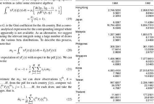
Table 1 gives the estimated parameters of the beta distrib-utions obtained using the procedure described in Section 3.2. These estimated parameters provide meaningful income distri-butions, all of which are skewed and unimodal; however, the very large values ofpfor Japan (and, to a lesser extent, Thailand in 1988) appear out of place. Further investigation of Japan re-vealed that the EViews program used to perform the calcula-tions took numerous iteracalcula-tions to converge. Estimation ofqwas stable, but estimation ofpandbwas not stable. This instabil-ity did not appear to be a problem, however. The parameters
bandp were highly correlated, and alternative pairs of(b,p)
close to the convergence point led to virtually identical income distributions. For Singapore, the quite different parameter es-timates in 1988 and 1993 may be explained by the different sources of data. For Thailand, the data for both years are from
Table 1. Estimated Coefficients From Beta Distributions
1988 1993
Milanovic, but the 1988 data are for income, whereas the 1993 data are for expenditure.
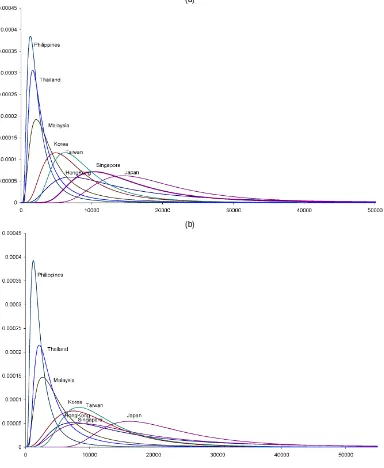
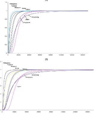
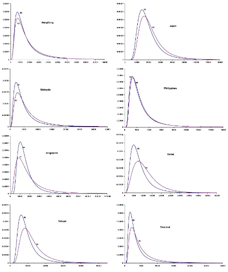
Figure 1 shows the plots of the density functions; they are consistent with general expectations. The locations of the distributions in terms of the mode and the mean appear to be ordered according to the real per capita incomes of these coun-tries. Also informative are the distribution functions and Lorenz curves for each country in each of the two years. To find these, we select a grid of income points(y1,y2, . . . ,yL)and compute
F(yi)=Byi/(b+yi)(p,q)andηi=Byi/(b+yi)(p+1,q−1).
Fig-ures 2(a) and 2(b) show the distribution functions for all of the countries in the study. Philippines, Thailand, Malaysia, Korea, and Taiwan appear to be consistently ranked from the poor-est to the richpoor-est. For any given income level, Philippines has the highest proportion of people whose incomes are below that level, followed by Thailand and then the other countries. The ranking of these countries remained unaltered over the two pe-riods. However, such a clear dominance pattern is not evident in the case of Japan, Singapore, and Hong Kong; for these three countries, the distribution functions cross over at some income levels. Figures 3(a) and 3(b) depict the Lorenz curves for Japan, Singapore, and Hong Kong. If interest centers on inequality only, with no concern for mean income, then these figures show clear Lorenz ordering, with Japan having the least inequality, followed by Singapore and Hong Kong.
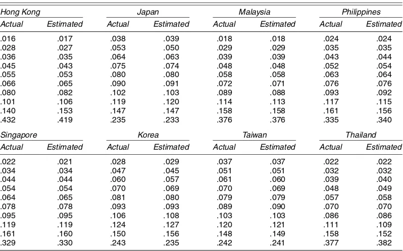
4.2 Goodness of Fit of Beta Distributions
It is useful to assess the goodness of fit of the beta distrib-utions by comparing the observed income shares with the
(a)
(b)
Figure 1. Cross-Country Distributions: (a) 1988; (b) 1993.
pected income shares derived using the estimated distributions. The empirical income shares are given by
gi= ciyi¯
N j=1cjy¯j
= cixi¯
N j=1cjx¯j
.
To find those implied by each beta distribution, we began with the population shares ci and corresponding cumulative
proportions
πi= i
j=1
cj,
and then found class limitsai(not necessarily the same as the
previously estimated class limits) such that
Ba
i/(bˆ+ai)(pˆ,qˆ)=πi.
We then found corresponding cumulative income shares from the first moment distribution function,
ˆ
ηi=
1 ˆ
µ
ai
0
yf(y)dy
= 1 ˆ
µ
ˆ pbˆ ˆ
q−1Bai/(bˆ+ai)(pˆ+1,qˆ−1)
=Ba
i/(bˆ+ai)(pˆ+1,qˆ−1).
The estimated income shares are given by
ˆ
gi= ˆηi− ˆηi−1.
Tables 2 and 3 compare the estimated and observed income shares. The actual (observed) and estimated (expected) income shares are remarkably similar for all of the countries in both years; in most cases the differences are in the third decimal
(a)
(b)
Figure 2. Cumulative Distribution Functions: (a) 1988; (b) 1993.
place. This outcome is very encouraging given that the parame-ters of the distributions have been estimated from limited data, and given that the class limitsaiimplied by the estimated pa-rameters, not theaigiving the “best fit,” were used to compute
the expected income proportions.
4.3 Temporal Analysis of Shifts in Income Distribution and Levels and Trends in Inequality
Figure 4 shows the density functions for 1988 and 1993 for each of the countries included in the current study.
Philip-(a) (b)
Figure 3. Selected Lorenz Curves: (a) 1988; (b) 1993.
Table 2. Income Shares 1988
Hong Kong Japan Malaysia Philippines
Actual Estimated Actual Estimated Actual Estimated Actual Estimated
.019 .020 .039 .039 .020 .020 .040 .039
.032 .031 .052 .051 .031 .031 .052 .053
.040 .039 .065 .065 .040 .040 .058 .059
.049 .048 .075 .075 .050 .050 .066 .067
.059 .058 .082 .083 .060 .061 .074 .075
.071 .071 .092 .093 .073 .073 .086 .086
.086 .087 .103 .104 .090 .090 .100 .099
.108 .111 .121 .122 .115 .115 .120 .117
.149 .156 .147 .147 .159 .158 .152 .149
.387 .380 .224 .221 .362 .362 .252 .256
Singapore Korea Taiwan Thailand
Actual Estimated Actual Estimated Actual Estimated Actual Estimated
.040 .039 .028 .030 .038 .038 .025 .025
.052 .052 .046 .044 .052 .051 .036 .035
.060 .061 .057 .054 .061 .061 .043 .044
.069 .070 .066 .064 .070 .069 .052 .052
.079 .079 .076 .075 .079 .079 .061 .062
.090 .090 .087 .087 .090 .090 .073 .074
.104 .103 .100 .102 .102 .103 .090 .089
.122 .120 .118 .123 .118 .120 .114 .112
.150 .147 .145 .155 .146 .148 .156 .152
.234 .237 .276 .265 .244 .241 .351 .355
NOTE: All shares are decile shares except for Japan and Philippines, where the population proportions were not equal for each class.
pines, Korea, and Taiwan are worthy of special mention. The in-come distribution in Philippines remained virtually unchanged over the period, whereas major structural shifts are evident in the case of Korea and Taiwan, which have been called the “Asian tigers” due to their performance during the study pe-riod.
The levels and trends in inequality can be studied using Gini coefficients and Lorenz curves. Both observed and estimated Gini coefficients are computed and presented. The observed values of the Gini coefficient were obtained by applying the
formula
G= N
i=1
ηi+1πi− N
i=1
ηiπi+1 (23)
to the grouped data, whereπiandηi are the observed
popula-tion and income shares. The estimated values were obtained by substituting estimatesbˆ,pˆ, andqˆinto the formula
G=2B(2p,2q−1)
pB2(p,q) . (24) Table 3. Income Shares 1993
Hong Kong Japan Malaysia Philippines
Actual Estimated Actual Estimated Actual Estimated Actual Estimated
.016 .017 .038 .039 .018 .018 .024 .024
.028 .027 .053 .050 .029 .029 .035 .035
.036 .035 .064 .063 .039 .039 .043 .044
.045 .043 .075 .074 .048 .048 .052 .054
.055 .053 .080 .080 .058 .058 .063 .064
.066 .065 .090 .091 .072 .071 .076 .076
.080 .082 .102 .103 .089 .088 .093 .092
.101 .106 .119 .120 .114 .113 .117 .115
.140 .153 .147 .147 .158 .158 .161 .156
.432 .419 .235 .233 .376 .376 .335 .340
Singapore Korea Taiwan Thailand
Actual Estimated Actual Estimated Actual Estimated Actual Estimated
.022 .021 .028 .029 .037 .037 .022 .022
.034 .034 .047 .045 .051 .051 .032 .032
.044 .044 .060 .057 .061 .060 .039 .040
.054 .054 .070 .069 .070 .069 .048 .049
.064 .065 .081 .080 .079 .079 .057 .058
.078 .078 .093 .093 .089 .090 .070 .070
.095 .095 .106 .108 .103 .103 .086 .086
.119 .119 .124 .127 .120 .121 .111 .109
.161 .160 .150 .156 .148 .149 .158 .152
.329 .330 .243 .235 .242 .241 .377 .382
NOTE: All shares are decile shares except for Japan, where the population proportions were not equal for each class.
Figure 4. Shifts in the Distributions Over Time.
The observed and estimated Gini coefficients for all countries are presented in Table 4. Overall, the estimated Gini coefficients are higher than the observed ones. This outcome is expected because the Gini coefficients estimated from the beta distribu-tion take into account the distribudistribu-tion of income within classes. The trends in inequality shown in Table 4 are also interesting. With the exception of Korea, inequality within each country in-creased over the period 1988–1993. This result is consistent with the general notion that inequality may increase in coun-tries experiencing rapid growth. The only surprising result is for
Singapore, where the Gini coefficient increased significantly. However, the two coefficients may not be directly comparable, because the data for the year 1993 were drawn from Milanovic (referring to income data), whereas the 1988 data were drawn from the ILO and refer to the expenditure distribution.
Besides comparing the Gini coefficients, we examined the Lorenz dominance properties of the estimated income distribu-tions for the years 1988 and 1993 using a sufficient condition described by Wilfling (1996). A distribution function F(y)is said to exhibit less inequality in the Lorenz sense than a
Table 4. Observed and Estimated Gini Coefficients
1988 1993
Observed Estimated Observed Estimated
Hong Kong .4598 .4755 .4974 .5168
Japan .2409 .2453 .2428 .2483
Malaysia .4474 .4607 .4629 .4773
Philippines .4001 .4064 .4181 .4293
Singapore .2858 .2911 .4167 .4276
Korea .3351 .3442 .3097 .3170
Taiwan .2903 .2972 .2931 .2996
Thailand .4254 .4381 .4559 .4704
Region .4732 .4818 .4718 .4802
butionH(y),F≤LH, if the Lorenz curve ofFis greater than
(lies above) or equal to the Lorenz curve ofH. Given that the income distributions of countryi andj follow a beta distribu-tion, then a sufficient condition for the income distribution of country ito Lorenz-dominate (i.e., have less inequality) than that for countryjis (Wilfling 1996)
pj≤pi and qj≤qi.
It is possible to draw conclusions on Lorenz dominance based on the foregoing sufficient condition. Comparing esti-mated values of p and q for 1988 and 1993 shows that the distribution in 1988 Lorenz-dominates that in 1993 for Hong Kong, Japan, Malaysia, Philippines, Singapore, and Thailand. The sufficient condition is not satisfied for Korea and Taiwan. It is also possible to use this condition to assess dominance across countries. For example, Taiwan Lorenz-dominates Malaysia in both 1988 and 1993. Japan, Singapore, and Korea provide a Lorenz ordering, as shown in Figure 3.
The results reported for each country demonstrate the feasi-bility of using the beta-2 distribution to model the distribution of income for the chosen Asian countries. The estimation pro-cedure discussed in Section 3.2 provides a method for estimat-ing the parameters of the distribution usestimat-ing grouped data in the form of population shares and class mean incomes. Results on
the levels and trends of inequality are meaningful and support the general notion that inequality within countries increased over the period 1988–1993. The next section focuses on in-equality in the region as a whole.
4.4 Regional Inequality
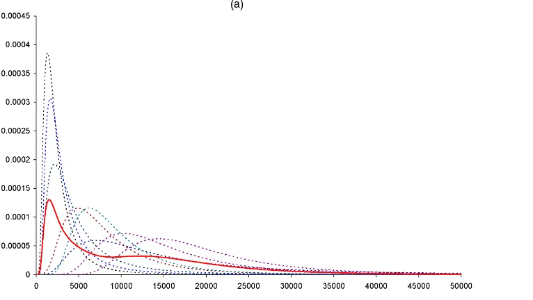
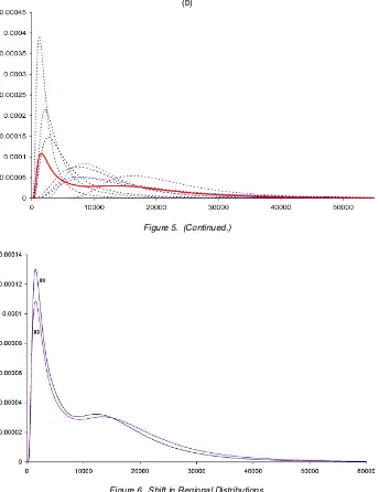
Figure 5 gives the 1988 and 1993 regional income distribu-tions, which appear as weighted averages of the income distri-butions for each country. For both years, the regional income distributions exhibit some degree of bimodality. The apparent reason for the second mode toward the right tail is the relatively large population of Japan, leading to the assignment of a rel-atively large weight to Japan’s distribution, coupled with the fact that the modes of its distributions are to the right of those for other countries. For comparative purposes, Figure 6 presents the 1988 and 1993 regional income distributions together in one graph. There is no obvious shift in the regional distributions.
Figure 7 shows the regional Lorenz curves for 1988 and 1993. The curves are virtually identical; visually, no difference can be detected in the figure. As expected, the regional Gini coef-ficients calculated using (21) are also almost identical, .4818 for 1988 and .4802 for 1993.
5. CONCLUSION
The main objective of this article was to suggest improve-ments to current approaches used for estimating global and re-gional inequality. We used an income distribution specification that is more general than the lognormal distribution that has been used in past research, and at the same time relaxed the as-sumption of a uniform distribution of income within (quintile and decile) population groups. In addition, we described a tech-nique for estimating the parameters of the beta-2 distribution when only limited data in the form of population shares and class mean incomes for groups of the population are available. The empirical illustration comprises eight East Asian countries
(a)
Figure 5. Regional Income Distributions as the Weighted Average: (a) 1988; (b) 1993. The dotted lines are country income distributions; the solid lines are the weighted average regional income distribution.
(b)
Figure 5. (Continued.)
Figure 6. Shift in Regional Distributions.
with income distribution data are for 1988 and 1993. The em-pirical results demonstrate the technique’s feasibility, and the goodness-of-fit results support its usefulness. The article also focused on the derivation of regional income distributions using country-specific distributions. Properties of the regional distrib-ution were examined by expressing the distribdistrib-ution as a mixture of the income distributions of each country. Levels and trends in inequality in these countries and the region were examined, and properties based on Lorenz dominance were established. The empirical results show a clear increase in inequality in most of the East Asian countries over the period 1988–1993.
Several avenues for further research appear promising. Based on the technique developed herein, the next step will be to use the methodology on a larger scale to derive improved estimates of inequality for the world, and for more recent years for which data may become available. Future work will also focus on derivating analytical properties of the mixture distribution used to study regional inequality.
Figure 7. Regional Lorenz Curves, 1988 and 1993.
108
Jour
nal
of
Business
&
Economic
Statistics
,
J
an
uar
y
2007
APPENDIX A: DATA ON POPULATION SHARES AND CLASS MEAN INCOMES
Table A.1. Population Shares and Class Mean Income, 1988
Japan Philippines Singapore
Population share (ci)
Class mean income (x¯i)
Population share (ci)
Mean income (¯xi)
Population share (ci)
Mean income (x¯i)
Population share (ci)
Income share (gi)
Hong Kong Malaysia South Korea Taiwan Thailand
10.0 969.0 47.0 783,279.6 30,171.4 4,110.7 8.6 73,915.5 13.7 1,781.2 10.0 2.2
10.0 1,632.0 75.0 1,276,662.2 41,341.0 5,800.5 8.9 943,925.2 12.4 2,581.5 10.0 3.5
10.0 2,040.0 97.0 1,574,921.7 48,631.9 7,035.3 9.9 1,069,767.4 11.2 3,187.7 10.0 4.5
10.0 2,499.0 119.0 1,850,881.4 55,736.0 8,367.7 10.2 1,184,573.0 10.5 3,829.0 10.0 5.5
10.0 3,009.0 145.0 2,118,479.7 63,156.7 9,895.0 10.2 1,309,333.3 9.9 4,564.2 10.0 6.6
10.0 3,621.0 176.0 2,416,738.2 71,286.6 11,844.7 10.2 1,456,919.1 9.6 5,493.7 10.0 8.0
10.0 4,386.0 217.0 2,790,260.5 81,423.1 14,525.6 10.2 1,642,487.0 9.2 6,714.2 10.0 9.7
10.0 5,508.0 275.0 3,289,217.0 94,181.8 18,506.4 10.5 1,879,487.2 8.7 8,440.7 10.0 12.2
10.0 7,599.0 381.0 4,047,409.4 115,827.9 25,298.0 10.6 2,253,846.2 8.1 11,422.9 10.0 16.3
10.0 19,788.0 869.0 7,698,998.7 194,204.2 57,095.2 10.8 3,375,314.9 6.7 22,856.7 10.0 31.6
Total population (S) 5,626,600 17,144,390 42,031,000 19,357,000 53,687,208 122,610,000 59,369,000
Mean income (y¯) 19,774.3 5,746.4 8,714.8 9,843.6 4,015.4 20,118.6 2,920.5
NOTE: Data onciandx¯iare drawn from work of Milanovic (2002a). These are used only in determining income shares in each of the decile groups. Data forSandy¯are from PWT6.1. The PTW income data are used in calculating average income,y¯i, in theith decile
group.
Table A.2. Population Shares and Class Mean Income, 1993
Japan
Population share (ci)
Class mean income (x¯i) Population
share (ci)
Class mean income (x¯i)
Hong Kong Malaysia South Korea Taiwan Thailand Singapore Philippines
10.0 1,600.0 879.0 1,493,547.1 56,662.5 4,718.4 182.0 3,116.5 8.6 917,603.0
10.0 2,800.0 1,403.1 2,563,469.9 77,749.4 6,694.8 287.0 4,487.6 8.9 1,248,275.9
10.0 3,600.0 1,846.3 3,231,492.8 92,186.6 7,035.3 369.0 5,548.8 9.7 1,364,741.6
10.0 4,500.0 2,286.0 3,801,756.2 106,145.3 8,318.4 453.0 6,691.0 10.2 1,508,620.7
10.0 5,500.0 2,793.9 4,388,312.9 120,442.6 10,042.8 541.0 8,029.7 9.9 1,676,880.2
10.0 6,600.0 3,422.9 5,034,611.4 136,289.6 12,034.8 659.0 9,717.1 10.1 1,869,209.8
10.0 8,000.0 4,246.9 5,740,651.9 156,443.0 14,659.2 799.0 11,904.7 10.2 2,088,235.3
10.0 10,100.0 5,435.0 6,718,246.3 182,645.8 18,132.0 1,000.0 15,034.3 10.4 2,380,952.4
10.0 14,100.0 7,547.6 8,168,344.8 225,716.0 23,492.4 1,354.0 20,619.4 10.7 2,855,643.0
10.0 43,200.0 17,996.0 13,170,369.7 368,717.1 33,236.4 2,767.0 42,820.5 11.3 4,352,644.8
Total population (S) 5,901,000 19,609,110 44,195,000 20,848,250 58,064,000 3,315,000 67,092,660 124,670,000
Mean income (y¯) 24,292.8 7,606.4 11,717.3 13,211.1 5,832.1 20,761.3 2,884.6 22,906.2
NOTE: Data onciandx¯iare drawn from work of Milanovic (2002a). These are used only in determining income shares in each of the decile groups. Data forSandy¯are from PWT6.1. The PTW income data are used in calculating average incomey¯iin theith decile
group.
APPENDIX B: ESTIMATION USING THE LOGNORMAL DISTRIBUTION
Suppose thatYis lognormal with parametersµandσ2, den-sity functionf(y), and distribution functionF(y). Then
where(·)=cdf of the standard normal distribution. The mo-ment conditions for the population shares, corresponding to (6) and (8), can be written as
ci=
ai
ai−1
f(y)dy+εi=F(ai)−F(ai−1)+εi. (B.1)
For the class mean incomes, we recognize that if income is distributed as lognormal with parameters µ andσ2, then the income share η or first moment distribution, F1(x), is also a lognormal distribution with parameters µ+σ2 and σ2 (see Aitchison and Brown 1957, p. 12), that is,
F1(x)=
Then the moment conditions corresponding to (7) and (9) can be written as
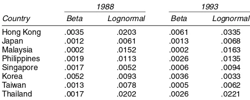
We estimated the parameters of the lognormal distributions along the lines described in Section 3.2. We obtained estimated income shares from the estimated lognormal distributions us-ing a procedure analogous to that described in Section 4.2 and compared the observed income shares with the estimated in-come shares. To compare the relative performance of the beta and lognormal distributions, we obtained root mean squared er-rors, which are reported in Table B.1. With the exception of Korea in 1993, in all cases the performance of the beta distrib-ution was far superior to that of the lognormal distribdistrib-ution.
Table B.1. Root Mean Squared Errors for Income Share Predictions
1988 1993
Country Beta Lognormal Beta Lognormal
Hong Kong .0035 .0203 .0061 .0335
Japan .0012 .0061 .0013 .0068
Malaysia .0002 .0152 .0002 .0163
Philippines .0019 .0113 .0026 .0135
Singapore .0017 .0052 .0006 .0094
Korea .0052 .0093 .0036 .0033
Taiwan .0013 .0078 .0005 .0062
Thailand .0017 .0202 .0026 .0221
[Received February 2005. Revised February 2006.]
REFERENCES
Aitchison, J., and Brown, J. A. C. (1957),The Lognormal Distribution, Cam-bridge, U.K.: Cambridge University Press.
Bandourian, R., McDonald, J. B., and Turley, R. S. (2002), “A Comparison of Parametric Models of Income Distribution Across Countries and Over Time,” mimeo, Brigham Young University.
Bhalla, S. S. (2002),Imagine There Is No Country, Washington: Institute for International Economics.
Bourguignon, F., and Morrisson, C. (1999), “The Size Distribution of Income Among World Citizens: 1820–1990,” mimeo, DELTA, Paris.
Chotikapanich, D., and Prasada Rao, D. S. (1998), “Inequality in Asia 1975–1990: A Decomposition Analysis,”The Asia Pacific Journal of Eco-nomics and Business, 2, 63–78.
Chotikapanich, D., Valenzuela, M. R., and Prasada Rao, D. S. (1997), “Global and Regional Inequality in the Distribution of Income: Estimation With Lim-ited/Incomplete Data,”Empirical Economics, 20, 533–546.
Creedy, J., and Martin, V. L. (eds.) (1997),Nonlinear Economic Models: Cross-Sectional, Time Series and Neural Network Applications, Cheltenham, U.K.: Edward Elgar.
Deininger, K., and Squire, L. (1996), “Measuring Inequality: A New Data Base,” mimeo, The World Bank, Washington, DC.
Dowrick, S., and Akmal, M. (2001), “Contradictory Trends in Global In-equality: A Tale of Two Biases,” available athttp://ecocomm.anu.edu.au/ economics/staff/dowrick/dowrick.html.
Dowrick, S., Eckland, R., and Freyens, B. (2004), “Global Poverty Measure-ment: Why PPP Methods Matter,” presented at the 28th General Conference of the International Association for Research in Income and Wealth, Au-gust 22–28, 2004, Cork, Ireland.
International Labour Office (1995),Household Income and Expenditure Statis-tics, 1997–1991, No. 4, Geneva: International Labour Office.
Kleiber, C., and Kotz, S. (2003),Statistical Size Distributions in Economics and Actuarial Sciences, New York: Wiley.
Lambert, P. J. (1993), The Distribution and Redistribution of Income, Manchester, U.K.: Manchester University Press.
McDonald, J. B. (1984), “Some Generalized Functions of the Size Distribution of Income,”Econometrica, 52, 647–663.
McDonald, J. B., and Ransom, M. R. (1979), “Functional Forms, Estimation Techniques and the Distribution of Income,”Econometrica, 6, 1513–1525. McDonald, J. B., and Xu, Y. J. (1995), “A Generalization of the Beta
Distrib-ution With Applications,”Journal of Econometrics, 66, 133–152; errata, 69, 427–428.
Milanovic, B. (2002a), “True World Income Distribution, 1988 and 1993: First Calculations Based on Household Surveys Alone,”The Economic Journal, 112, 51–92.
(2002b), “The Ricardian Vice: Why Sala-i-Martin’s Calculations of World Income Inequality Are Wrong,” available at SSRN:http://ssrn.com/ abstract=403020.
(2002), “One-Third of the World’s Growth and Inequality,” Discussion Paper 2002/38, WIDER, United Nation University.
Sala-i-Martin, X. (2002a), “The Disturbing Rise of Global Income Inequality,” Working Paper 8904, National Bureau of Economic Research, pp. 1–75.
(2002b), “The World Distribution of Income (Estimated From Individ-ual Country Distributions),” Working Paper 8905, National Bureau of Eco-nomic Research, pp. 1–68.
Slottje, D. J. (1984), “A Measure of Income Inequality in the U.S. for the Years 1952–1980 Based on the Beta Distribution of the Second Kind,”Economic Letters, 15, 369–375.
(1987), “Relative Price Changes and Inequality in the Size Distribu-tion of Various Components of Income,”Journal of Business & Economic Statistics, 5, 19–25.
Theil, H. (1989), “The Development of International Inequality, 1960–1985,”
Journal of Econometrics, 42, 145–155.
Wilfling, B. (1996), “Lorenz Ordering of Generalized Beta-II Income Distribu-tions,”Journal of Econometrics, 71, 381–388.