LEAST SQUARE SUPPORT VECTOR MACHINE FOR DETECTION OF
TEC-SEISMO-IONOSPHERIC ANOMALIES ASSOCIATED WITH THE POWERFUL
NEPAL EARTHQUAKE (M
w=7.5) OF 25 APRIL 2015
M. Akhoondzadeh
Remote Sensing Department, School of Surveying and Geospatial Engineeringl, University college of Engineering, University of Tehran, North Amirabad Ave., Tehran, Iran - [email protected]
Commission VIII, WG VIII/1
KEY WORDS: Ionosphere, TEC, earthquake, anomaly, LSSVM.
ABSTRACT:
Due to the irrepalable devastations of strong earthquakes, accurate anomaly detection in time series of different precursors for creating a trustworthy early warning system has brought new challenges. In this paper the predictability of Least Square Support Vector Machine (LSSVM) has been investigated by forecasting the GPS-TEC (Total Electron Content) variations around the time and location of Nepal earthquake. In 77 km NW of Kathmandu in Nepal (28.147°N, 84.708°E, depth=15.0 km) a powerful earthquake of Mw=7.8 took place at 06:11:26 UTC on April 25, 2015. For comparing purpose, other two methods including
Median and ANN (Artificial Neural Network) have been implemented. All implemented algorithms indicate on striking TEC anomalies 2 days prior to the main shock. Results reveal that LSSVM method is promising for TEC sesimo- ionospheric anomalies detection.
1. INTRODUCTION
The pre-seismic disturbances occurring in lithosphere, atmosphere and ionosphere in absence of significant solar and geomagnetic perturbations are usually considered as earthquake precursors.
The ionospheric anomalies usually take place in the D, E and F layers, and may be observed 1 to 10 days prior to the earthquake and continue a few days after it. Many papers and reports have been published on satellite observations of the ionospheric plasma, the flux of charged particles, the DC electric field, electromagnetic waves and geomagnetic field associated with seismic activity (Parrot, 1995; Liu et al., 2004; Hayakawa and Molchanov, 2002; Pulinets and Boyarchuk, 2004; Akhoondzadeh, 2011). The pre-earthquake disturbances usually affect the TEC (Total Electron Content). In this study, GPS-TEC data have been downloaded via NASA Jet Propulsion Laboratory (JPL) website. Global Ionospheric Map (GIM) data constructed from a 5° × 2.5° (Longitude, Latitude) grid with a time resolution of 2 hours.
The accurate anomaly detection in time series of earthquake precursors is regarded as one of the most challenging tasks since the behaviors of precursors is complicated, dynamic and nonlinear. In addition, the affected factors in ionospheric precursors such as solar and
geomagnetic indices intensify the complexity of the ionospheric precursors.
As a modified version of Support Vector Machine (SVM), Least Square SVM (LSSVM) was proposed by Suykens and Vandewalle in 1999. It retains principle of the Structural Risk Minimization (SRM) and has important improvement of calculating speed with traditional SVMs (Wang and Shang, 2014). It is because of changing inequality constraints into equations and takes a squared loss function. Therefore, LSSVM solves a system of equations instead of a quadratic programming problem. Due to the mentioned advantages of LSSVM, it has been implemented as a classification model (Wang and Shang, 2014). In this paper the predictability of LSSVM has been investigated by predicting the GPS-TEC variations around the time and location of Nepal earthquake.
2. LSSVM METHOD
proposed by Suykens and Vandewalle in 1999 to overcome these shortcomings.
Unlike the classical neural networks approach, SVM formulates the statistical learning problem as a quadratic programming with linear constraints, by the use of nonlinear kernels, high generalization ability, and sparseness of solution. However, for large-scale problems, the optimization process of SVM has high computational complexity, due to the high-dimensional matrix involved in the quadratic programming whose size is directly proportional to the training sample size (Zhou et al., 2011). LS-SVM needs significantly less training effort than the standard SVM as a result of the model simplification.
The basic principle of SVM regression is to estimate the respectively (Zhou et al., 2011).
Given a sample of training data
{
(
x
iy
i)
}
iN 1,
= , LS-SVM determines the optimal weight vector and bias term by minimizing the following cost function, R,2
subject to the equality constraints
N
function regularizes weight sizes and penalizes large weights. Therefore, the weights tend to converge to similar values in that large weights cause excessive variance and hence deteriorate the generalization ability of LSSVM (Suykens and Vandewalle, 1999; Zhou et al., 2011). The second part of Eq. (2) considers the regression error of all training data. The regularization parameter c controls the trade-off between the bias and variance of LS-SVM model. Note that the LSSVM model has equality constraintsconsidered in the objective function of LS-SVM model, while the standard SVM model has a linear combination of slack variables in its objective function. These two modifications simplify the quadratic optimization problem for the standard SVM to be linear for LSSVM (Suykens and Vandewalle, 1999; Zhou et al., 2011).
The Lagrangian of Eq. (2) is Kuhn–Tucker Theorem, the conditions of optimality are (Suykens and Vandewalle, 1999; Zhou et al., 2011)
0
linear equations after eliminating w and e,(7)
In this study Gaussian kernel function has been used.
).
determining the width of Gaussian kernel.To implement the LSSVM method, training and testing data were initially set respectively to 60% and 40% of all TEC data. The input patterns in the LSSVM method are,
x4=f(x1, x2, x3)
At each step, using the training data, the LSSVM method is implemented and the prediction error (PE) can be written as: the LSSVM method, respectively.
Finally, the TEC value is predicted and then is compared to the true value in testing set. In the case of testing process, if the value of DXi (i.e. the difference between the actual
Dst and F10.7) were used to distinguish seismic anomalies
from the other anomalies related to the geomagnetic and solar activities. Figure 1 illustrates the variations of Kp,
Ap, Dst and F10.7 indices, during the period of 01 March
to 30 April 2015. An asterisk indicates the earthquake time. The X-axis represents the days relative to the earthquake day. The Y-axis represents the universal time coordinate.
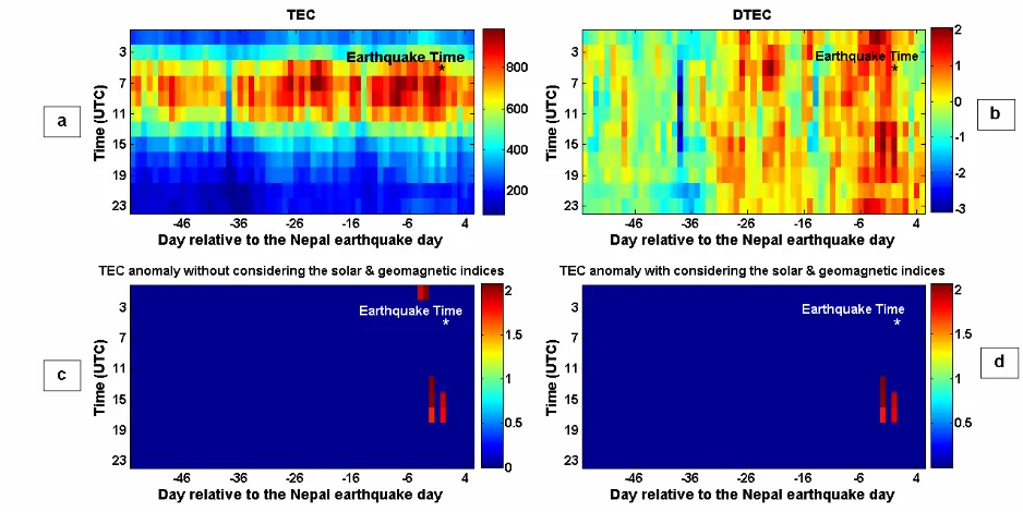
Figure 2(a) shows TEC variations during the period of 01 March to 30 April 2015. To implement the Median method, Dx which will be called DTEC here, is calculated using Eq. (11). parameter value, higher bound, lower bound, median value, Interquartile range and differential of x, respectively. According to this, if the absolute value of Dx would be and geomagnetic indices. Then to distinguish pre-earthquake anomalies from the other anomalies related to the geomagnetic activities, the five conditions of
75
Dst
,Ap
<
10
and F10.7 <150, respectively, are jointly used using AND operator to construct the anomaly map (Figure 2(d)). The TEC value exceeds the higher bound (M
+
1
.
75
×
IQR
), 2 days before the earthquake time at 14:00, 16:00 and 18:00 UTC with the values of 18.68 %, 15.97% and 0.32% of the higher bound, respectively. It is seen that the other detected anomalies in Figure 2(c) have been masked by high geomagnetic activities (Figure 2(d)). In figure 2(d) increases (08.40% and 04.13%) in TEC are clearly observed at 16:00 and 18:00 UTC on earthquake date (Table 2).Fig. 1. a), b), c) and d) show respectively, the variations of Kp, Ap, Dst and solar radio flux (F10.7) indices during the period of
01 March to 30 April 2015. An asterisk indicates the earthquake time. The X-axis represents the days relative to the Nepal earthquake day.
To implement the Artificial Neural Network (ANN) method (Akhoondzadeh, 2013), training data were set to 60% of all data. Using the training data, the pattern vectors in feature space are constructed. In the case of testing process, if the difference value PEi between the actual value Xi and the
predicted value
X
ˆ
i , is outside the pre-defined boundsµ
±
2
.
0
×
σ
, (µ
andσ
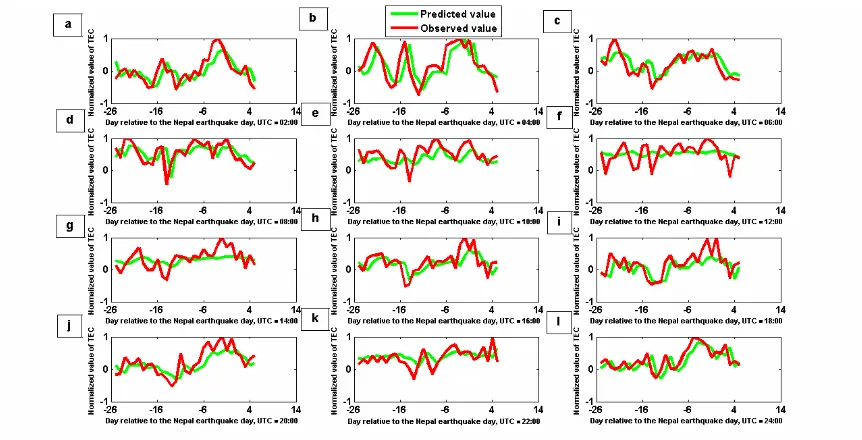
are the mean and the standard deviation of PEivalues) the anomaly is detected.Red and green curves in figures 3(a) through (l) represent the observed and the predicted TEC values using the ANN method, respectively during the days selected as training and testing set. These figures indicate that the ANN method is a good estimator for non linear time series such as TEC variations. It can be seen that the ANN method efficiently predicts values during the time of testing.
Figures 4(a) through (l) represent the differences between the observed and the predicted TEC values during the testing data using the ANN method. Figure 5(a) is a representation of the differences values during the testing set. Figure 5(b) shows the DTEC values obtained from Then to distinguish pre-earthquake anomalies from the other anomalies related to the geomagnetic activities, the five conditions of
DTEC
>
2
.
0
,Kp
<
2.5
,F10.7
<
respectively, are jointly used using AND operator to construct the anomaly map (Figure 5(d)). The DTEC value exceeds the upper bound (µ
+
2
.
0
×
σ
) with the values of 8.14%, 2 days before the earthquake at 14:00 UTC, and also 4 days after the earthquake time at 22:00 UTC with the value of 38.49% (Table 2).To implement the LSSVM method, training data were set to 60% of all data. Using the training data, the pattern vectors in feature space are constructed. In the case of testing process, if the difference value PEi between the
actual value Xi and the predicted value
X
ˆ
i, is outside thepre-defined bounds
µ
±
2
.
0
×
σ
, (µ
andσ
are the mean and the standard deviation of PEivalues) the anomalyis detected.
Red and green curves in figures 6(a) through (l) represent the observed and the predicted TEC values using the LSSVM method, respectively during the days selected as training and testing set.
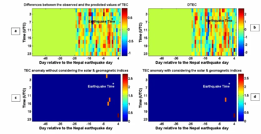
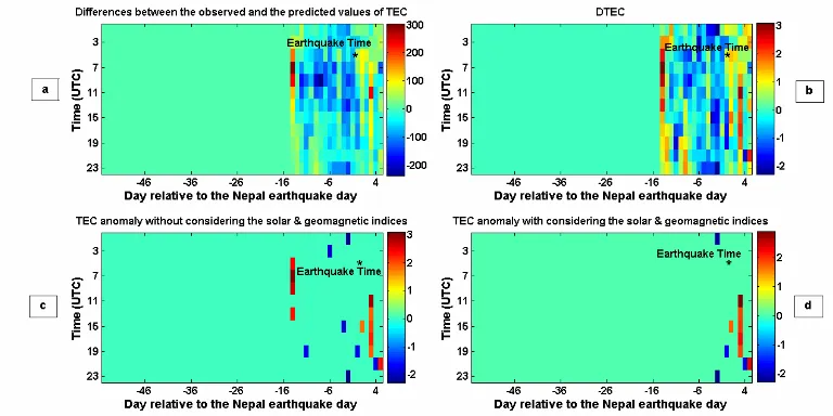
Figures 7(a) through (l) represent the differences between the observed and the predicted TEC values during the testing data using the LSSVM method. Figure 8(a) is a representation of the differences values between the observed and predicted values during the testing set. Figure 8(b) shows the DTEC values obtained when
DTEC
>
2
.
0
. Then to distinguish pre-earthquake anomalies from the other anomalies related to the geomagnetic activities, the five conditions of0
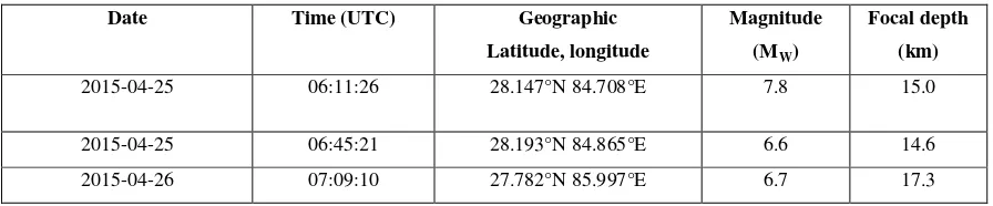
24:00 UTC, and also with the value of -0.5%, on earthquake date atTable 1. Characteristics of the Nepal earthquake and its main after shocks (reported by http://earthquake.usgs.gov/).
Date Time (UTC) Geographic
Table 2. The main detected anomalies for Nepal earthquake using the implemented methods. Value is calculated
by
p
=
±
100
×
(
Dx
−
k
)
/
k
. Day is relative to the earthquake day.Method Day Time (UTC) Value %
Median 0
-2
16:00; 18:00 14:00; 16:00; 18:00
8.40; 4.13 18.68; 15.97; 0.32
ANN -2
+4
14:00 22:00
8.14 38.49
LSSVM -2
0 +1 +3 +4 +5
2:00; 24:00 20:00 16:00
12:00; 14:00; 16:00; 18:00; 20:00 22:00
22:00
-26.18; 30.89 0.5 0.71
67.20; 9.10; 15.45; 26.61; 7.89 -1.8
30.89
Fig. 4. a) through l) Variations of the differences between the observed and the predicted values of TEC obtained from ANN method on days selected as testing set at different universal times. The red horizontal lines indicate the upper and lower bounds (
µ
±
2
×
σ
). The green horizontal line indicates the mean value (µ
). The X-axis represents the day relative to the Nepal earthquake day.Fig. 6. a) through l) Variations of the observed (red curve) and predicted (green curve) TEC values obtained from LSSVM method during at different universal times. The X-axis represents the day relative to the Nepal earthquake day.
Fig. 8. a) Differences between the observed and the predicted values of TEC obtained from LSSVM method. b) DTEC variations. c) Detected anomalies using LSSVM method without considering the geomagnetic indices. d) Detected anomalies using LSSVM method with considering the geomagnetic indices. The X-axis represents the days relative to the Nepal earthquake day. The Y-axis represents the universal time coordinate.
20:00 UTC. Other post-seismic anomalies could be associated with the strong aftershocks (Table 1).
4. CONCLUSIONS
This paper attempts to acknowledge the ability of LSSVM as a good predictor to forecast the GPS-TEC variations around the time and location of Nepal earthquake. Also two classical and intelligent methods including Median and ANN have been implemented. Using all applied methods prominent TEC anomalies are observed 2 days prior to the main shock. Results reveal that LSSVM method is promising for TEC sesimo- ionospheric anomalies detection.
ACKNOWLEDGEMENT
The author would like to acknowledge the NASA Jet Propulsion Laboratory for the TEC data and solar-geomagnetic indices.
REFERENCES
Akhoondzadeh, M., 2011. Comparative study of the earthquake precursors obtained from satellite data. PhD thesis, University of Tehran, Surveying and Geomatics Engineering Department, Remote Sensing Division. Akhoondzadeh, M., 2013. A MLP neural network as an investigator of TEC time series to detect
seismo-ionospheric anomalies. Advances in Space Research, 51, pp. 2048-2057.
Hayakawa, M., and Molchanov, O.A., 2002. Seismo- Electromagnetics: Lithosphere-Atmosphere-Ionosphere Coupling. Terra Scientific Publishing Co. Tokyo, 477. Liu, J.Y., Chuo, Y.J., Shan, S.J., Tsai, Y.B., Pulinets, S.A., and Yu, S.B., 2004. Pre-earthquake-ionospheric anomalies registered by continuous GPS TEC. Ann. Geophys., 22, pp. 1585-1593.
Parrot, M., 1995. Use of satellites to detect seismo-electromagnetic effects, Main phenomenological features of ionospheric precursors of strong earthquakes. Advances in Space Research, 15 (11), pp. 1337-1347.
Pulinets, S. A., and Boyarchuk, K.A., 2004. Ionospheric Precursors of Earthquakes. Springer, Berlin.
Suykens, J. A. K., Vandewalle, J., 1999. Least squares support vector machine classifiers. Neural processing letters, 9 (3), pp. 293-300.
Wang, S., and Shang, W., 2014. Forecasting Direction of China Security Index 300 Movement with Least Squares Support Vector Machine. Procedia Computer Science, 31, pp. 869-874.