REAL-TIME STREAM PROCESSING FOR ACTIVE FIRE MONITORING ON
LANDSAT 8 DIRECT RECEPTION DATA
C. Böhme a, *, P. Bouwer a, MJ. Prinsloo a
a Pinkmatter Solutions, Pretoria, South Africa – (chris, philip, thinus)@pinkmatter.com
KEY WORDS: Real-time Processing, Near-real-time processing, NRT, Fire Detection, Fire Notification, Landsat 8
ABSTRACT:
Some remote sensing applications are relatively time insensitive, for others, near-real-time processing (results 30-180 minutes after data reception) offer a viable solution. There are, however, a few applications, such as active wildfire monitoring or ship and airplane detection, where real-time processing and image interpretation offers a distinct advantage. The objective of real-time processing is to provide notifications before the complete satellite pass has been received. This paper presents an automated system for real-time, stream–based processing of data acquired from direct broadcast push-broom sensors for applications that require a high degree of timeliness. Based on this system, a processing chain for active fire monitoring using Landsat 8 live data streams was implemented and evaluated. The real-time processing system, called the FarEarth Observer, is connected to a ground station’s demodulator and uses its live data stream as input. Processing is done on variable size image segments assembled from detector lines of the push broom sensor as they are streamed from the satellite, enabling detection of active fires and sending of notifications within seconds of the satellite passing over the affected area, long before the actual acquisition completes. This approach requires performance optimized techniques for radiometric and geometric correction of the sensor data. Throughput of the processing system is kept well above the 400Mbit/s downlink speed of Landsat 8. A latency of below 10 seconds from sensor line acquisition to anomaly detection and notification is achieved. Analyses of geometric and radiometric accuracy and comparisons in latency to traditional near-real-time systems are also presented.
1 INTRODUCTION
1.1 The Landsat 8 mission
The Landsat Data Continuity Mission (LDCM) spacecraft was launched in February 2013 and is now managed by the US Geological Survey (USGS) as the Landsat 8 mission. The spacecraft carries two push-broom instruments, the Operational Land Imager (OLI) with 9 reflective bands as well as the Thermal Infrared Sensor (TIRS) with two thermal bands. Landsat 8 orbits the earth every 90 minutes and revisits the same 185km swath every 16 days (USGS, 2013a).
Although orthorectified image data is freely available from the USGS, Landsat 8 is a popular mission for direct reception by international ground stations. At the time of writing there are 14 operational receiving stations that receive Landsat 8 in their national interest for real-time access to the Landsat data (USGS, 2015).
1.2 Near-real-time and real-time processing
In typical near-real-time (NRT) processing chains production is started once the satellite pass is completed and all the data is received and transferred to a processing system. The European Space Agency (ESA) defines near-real-time data delivery for the Sentinel 1 mission as products that are delivered within 3 hours of acquisition. Quasi real-time delivery according to ESA is anything that is processed and delivered within 1 hour of acquisition (ESA, 2015).
For some applications, where timeliness is of great importance, even the latency incurred by waiting for an overpass to complete (in the order of 10 minutes for a typical polar orbiting satellite) can already be disadvantageous to an early warning system.
* Corresponding author
A technique is proposed to process data while it is received from the demodulator during a satellite overpass, referred to as a real-time, stream-based processing algorithm. This approach aims to achieve a very low latency between image acquisition and anomaly detection. Processing commences as soon as acquisition starts and completes shortly after the satellite pass is completed. To make this possible, some trade-offs between quality and speed are made that are highlighted in the next sections.
For comparison, the Landsat 8 processing system of the USGS takes between 30-60 minutes to perform radiometric and geometric correction of a ten minute satellite overpass. The stream-based approach outlined here and implemented in the FarEarth Observer system, aims to do this while the pass is still in progress (i.e. in under ten minutes).
1.3 Fire detection using reflective bands
Although Landsat 8 alone is not suitable for operational fire monitoring due to its 16-day revisit cycle, it is chosen as a platform to illustrate the real-time, stream-based processing approach with a fire detection use case.
It has been shown by Morisette et al that fire detection using only the near- and short-wave infrared bands is feasible (Morisette, 2005). The ratio and difference between the near-infrared and short-wave infrared bands is used along with threshold values and background radiation contrast.
= ��� − ��� ; � = ������ (1)
radiation is also taken into account to classify a pixel as a hotspot (Giglio, 2008). These values were empirically determined for Landsat 7 ETM+ by Schroeder et al and provide a starting point for values used for Landsat 8 OLI (Schroeder, 2008).
2 IMPLEMENTATION
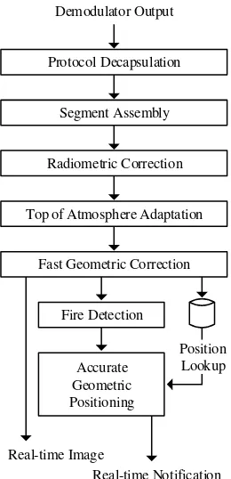
2.1 Stream-based processing approach
Unlike traditional satellite image processing approaches, where the whole image or scene is acquired before it is processed, stream-based processing starts while the data is being recorded and downlinked from the satellite. Processing is performed on segments assembled from the data stream. In this implementation a segment height of 800 pixels is used.
Protocol Decapsulation
Segment Assembly
Radiometric Correction
Top of Atmosphere Adaptation
Fast Geometric Correction
Fire Detection Demodulator Output
Real-time Notification Real-time Image
Accurate Geometric Positioning
Position Lookup
Figure 1. Process flow of stream-based processing
2.2 Protocol decapsulation
Landsat 8 uses data transfer standards developed by the Consultative Committee for Space Data Systems (CCSDS). To access real-time Landsat 8 OLI data from the demodulator output, decapsulation of the transport protocols is performed in software.
Figure 2 shows the protocol layers and order of processing that is performed (from top to bottom) to access raw image lines from the OLI sensor.
CCSDS Transfer Frame Layer (CCSDS 732.0) CCSDS Space Packet Layer (CCSDS 133.0) CCSD File Delivery Protocol Layer (CCSDS 727.0)
Raw OLI Mission Data
Figure 2. Landsat 8 data downlink protocol stack (USGS, 2010)
Figure 3. OLI image of Reno, California produced in real-time with band combinations 6-5-4.
2.3 Radiometric corrections
Several radiometric corrections are applied in real-time to the raw OLI data as data segments are received. Bias removal, response linearization, gain application and relative top of atmosphere corrections are applied. These corrections are simplified and other finer corrections ignored in order to strike a balance between accuracy and processing time.
The most recent valid Landsat 8 Calibration Parameter Files (CPF) and Response Linearization Look-up Tables (RLUT) are used as input. Bias Parameter Files (BPF) are however not used since these are updated daily, and would add complexity to the system while yielding only a slight gain in radiometric accuracy.
2.3.1 Bias removal: The raw OLI data contains a digital number (DN) value per pixel. The average bias value per detector is obtained from the CPF and applied to give bias-corrected DN values as output.
2.3.2 Response linearization: The latest RLUT, currently at version 9, is used to correct for the non-linear response of the detectors.
2.3.3 Gain application: Gain correction is performed using values taken from the CPF. The absolute gain is applied per sensor chip assembly (SCA) and the relative gain per individual detector.
2.3.4 Dropped frames, noise and striping: During standard level 1 processing, several more rigorous checks and corrections are performed in order to remove noise and striping artifacts. These corrections have a relatively small overall impact on the image quality and are ignored by the FarEarth Observer for the sake of processing efficiency.
For level 1 processing, a cyclic redundancy check (CRC) would normally be calculated on each frame, and faulty image lines filled with zeroes. Since this check is quite processing intensive, the FarEarth Observer ignores this check. Consequently, the line output may contain incorrect pixel values; conversely, valid pixels in a faulty line will also not be discarded.
Saturated pixels are not handled in any special way and the DN values are used as is, contrary to how a standard level 1 product would be affected. Impulse noise, which is random a-periodic noise that causes a pixel value to be notably different from that of its neighbouring pixels, is also not filtered.
The OLI BPF provides detector coefficients that can be used to estimate a more accurate bias variation for a given detector. However, since the FarEarth Observer does not use the BPF as input, it has to rely only on the CPF and RLUT values to remove detector striping artifacts.
2.3.5 Relative top of atmosphere: The bias-corrected, linearized and gain-corrected radiance values are converted to relative top of atmosphere (TOA) values. The earth-sun distance and sun angle is calculated for the segment and the reflective conversion constants are obtained from the CPF per band. These values are used to calculate the TOA values.
An adaptation of the USGS OLI radiometric algorithm is used by the FarEarth Observer to calculate the top of atmosphere values of the raw pixel data (USGS, 2013b), shown in Equation 2.
����,�,�= Λ �,�,� − �,��,� ∗ �,� � 2� �
sin � �,�,� (2)
where b, d and t is the band, detector and time of the specific pixel, Λ the response linearization function, is the raw detector output (digital number), the average bias factor as per the CPF, α the absolute gain value as per the CPF, the relative gain component as per the CPF, the earth-sun distance, μ the reflectance conversion constant, and θ the solar elevation.
2.4 Geometric corrections
Geometric correction is done using a systematic calculated sensor model. No digital elevation model (DEM) or ground control is used. The sensor model describes the line of sight (LOS) for each detector in each SCA for every band in geodetic latitude and longitude (USGS, 2013b). Additional input from the CPF, such as detector offset and SCA overlap, are incorporated in the LOS model to improve the accuracy.
Each detector pixel is projected on the ground using the line of sight model and a position average to get an approximate centre latitude and longitude. The Universal Transverse Mercator (UTM) zone for this centre coordinate is determined and used to project all detector pixels to UTM. The nadir ground sampling distance (GSD) for OLI reflective bands are 30 meters. With the detector pixel’s dimensions and coordinates now both in meters, an iterative fit is done to align the SCAs and bands of the different detectors.
The output from the geometric correction are simple vertical offsets describing the distance a pixel needs to shift down, relative to a reference detector. These offsets are assumed to stay constant over the entire pass, and are thus calculated only once at the start of a pass. As the pixel data is only shifted vertically, no resampling is done.
Although the above-mentioned process is sufficient to provide an at-a-glance view of the data, it is insufficient to provide accurate locations of interesting features such as fires. Therefore, in addition to the process described above, all attitude, ephemeris and sample timestamps are kept in system memory. This allows for a quick calculation of the exact locations of a pixel, when required. This lookup was also used to calculate the geometric accuracy described later in this paper (see section 3.1).
During normal level 1 processing, all ancillary data would be filtered and outliers rejected. During stream-based processing, this is not possible as not all ancillary data is available at the time a segment is processed. Instead, a linear interpolation between ancillary samples is done which causes small inaccuracies in the LOS model.
2.5 Hotspot detection
Hotspot detection is performed as a proof of concept for real-time radiometric pixel classification. The threshold values set out by Schroeder et al for Landsat 7 ETM+ are used.
Hotspots and hotspot candidates are determined radiometrically by exploiting the high degree of accuracy of the radiometric correction and band alignment (see sections 3.1.2 and 3.2). Once a pixel has been classified as a hotspot, the location of the hotspot is accurately determined by performing a lookup for the pixel’s location. This location lookup is relatively time consuming and hence is only performed when an anomaly (in this example a fire) is located. By only calculating an accurate geolocation for an anomaly and not for every pixel, the overall processing time and latency are kept within the desired range.
3 RESULTS
3.1 Geometric accuracy assessment
In order to assess the geometric accuracy of the stream-based processing system, an accuracy measurement based on pixel correlation between the USGS’s LPGS (Landsat Product Generation System) product and the FarEarth Observer product have been performed. Furthermore the band-to-band alignment of the stream-based product has been assessed.
3.1.1 Absolute geometric accuracy: An absolute geometric accuracy assessment has been performed by comparing a FarEarth Observer generated product against a reference L1G (Level 1 geometric) product produced by LPGS. The following table shows the residuals in both x and y directions.
Residuals in pixels Standard deviation
X direction 0.80 0.66
Y direction 0.73 0.44
Table 1. Geometric accuracy of a real-time product
Pixel-to-pixel accuracy between the reference image and a real-time image segment is visualized in Figure 4. Green pixels represent errors of less than half a pixel, cyan pixels errors less than one pixel, blue one to two pixel errors and yellow errors of more than two pixels. The chessboard pattern that can be
observed in Figure 4 reflects the OLI’s 14 detector assemblies and their relative offsets. The observed pattern is due to small errors introduced by imperfect detector alignment of the real-time processing algorithm.
Figure 4. Pixel offsets plotted against the reference product (green: error < 0.5, cyan: 0.5 < error < 1, blue: 1 < error < 2, yellow: error > 2 pixels)
3.1.2 Band-to-band alignment: Band-to-band alignment is especially important if algorithms based on band comparison or spectral classification are used in a real-time detection system. The following values are obtained by measuring mean and standard deviations of pixel residuals between the most commonly used OLI bands:
Table 2. Band-to-band mean (and standard deviation) pixel residuals in the horizontal direction (worst value in bold)
Blue Green Red NIR SWIR1 SWIR2
Table 3. Band-to-band mean (and standard deviation) pixel residuals in the vertical direction (worst values in bold)
It can be seen from the data above that the overall band misalignment is typically far less than 0.1 pixels in the x and y directions.
3.2 Radiometric accuracy assessment
A comparison of the radiometric quality of the output from the FarEarth Observer against Landsat 8 scenes produced by LPGS has been performed. Top of atmosphere reflectance values, corrected for solar incidence angle and scaled to a range between 0 and 10000, were compared against each other.
To counter for the effect of geometric differences, each product is segmented into 16 × 16 pixel tiles and the reflectance values averaged over each tile before they are compared. The mean and standard deviation of the difference in reflectance values are given in Table 4 below.
Band Standard
Table 4. Difference between TOA reflectance values (scaled to 10000) of a real-time product and a LPGS reference image
The absolute radiometric accuracy of the OLI sensor has been determined in-flight by the USGS to be around 4%, under the design criteria of 5% (Morfitt, 2014). An additional error of less than 0.3% can be considered negligible.
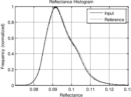
A histogram comparison, independent from geometric differences, is drawn between one of the candidate scenes and an LPGS-generated scene for band 2, shown in Figure 5 below. A slight shift along the reflectance scale can be observed.
Figure 5. Reflectance histogram of a real-time product compared to a LPGS-generated product.
3.3 Hotspot detection
Figure 6. Real-time Landsat 8 image (band combination 7-5-3)
Figure 7. Real-time generated fire mask for the above image (shown in pink)
Figure 6 and Figure 7 show bush fires over southern Tanzania with and without the generated fire mask.
Figure 8. Real-time Landsat 8 fire mask for fires near Adelaide, Australia on 4 January 2015
Figure 9. MODIS fire mask overlaid on the real-time Landsat image in the previous figure (dark pink: high confidence, light
pink: nominal confidence fire pixel)
The algorithm performs reasonably well to detect fire pixels at a 30m resolution. Some false positives are still detected over built-up areas with highly reflective roofs or areas with particularly bright patches of sand. The algorithm could benefit from tuning the threshold values determined for ETM+ to the OLI bands of Landsat 8.
3.4 Timeliness
The FarEarth Observer was built so as not to require any special hardware beyond an average personal computer. On such a device the processing time of a complete satellite pass including fire detection takes less time than the actual acquisition of the data on board the satellite. The algorithm can therefore be considered faster than real-time.
Latency, however, is incurred by the processing chain. The overall latency from data acquisition at the demodulator to the detection of the actual hotspot has been measured to be less than 10 seconds. About 40% of this is due to the segment assembly, i.e. buffering of the pixel data to assemble a complete segment. Smaller segments would significantly decrease latency. For non-pixel-based operations such as ship-wake detection, however, smaller segments create complexities with features distributed over multiple segment. For a fire detection scenario, a 10 second segment seems satisfactory, therefore a segment height of 800 pixels was chosen for these tests.
4 CONCLUSION
It was shown that real-time processing with a latency of less than 10 seconds can be achieved to detect wild fires with satisfactory accuracy. The real-time, stream-based processing approach lends itself well to monitoring applications of a time critical nature.
Future work on the FarEarth Observer will focus on real-time ship and ship wake detection using Landsat 8 and other optical sensors. A real-time approach to processing MODIS and VIIRS data for operational, real-time, low-latency fire monitoring will also be investigated.
ACKNOWLEDGEMENTS
This work was made possible to a large degree by the USGS by making their source code open to international collaborators, and providing detailed technical documentation describing the OLI sensor and the Landsat 8 spacecraft.
REFERENCES
ESA, 2015, SENTINEL-1 Observation Scenario, Frascati, Italy
https://sentinel.esa.int/web/sentinel/missions/sentinel-1/observation-scenario (25 Mar 2015)
Giglio, L., 2008, Active fire detection and characterization with the Advanced Spaceborne Thermal Emission and Reflection Radiometer (ASTER)
Morfitt, R., 2014, Radiometric Performance of Landsat 8, Sioux Falls, USA https://calval.cr.usgs.gov/wordpress/wp-content/uploads/14.007_JACIE_Morfitt_L8_Radiometric_Perfo rmance.pdf (25 Mar. 2015)
Morisette, J., 2005, Validation of the MODIS active fire product over Southern Africa with ASTER data. International Journal of Remote Sensing, 26, pp. 4239-4264
Schroeder, W., 2008, Validation of GOES and MODIS active fire detection products using ASTER and ETM+.
USGS, 2010, Landsat Data Continuity Mission (LDCM) Spacecraft-To-Ground Interface Control Document, 70-P58230P, Rev. C, Gilbert, USA.
USGS, 2012, Landsat Data Continuity Mission (LDCM) Mission Data Format Control Book (DFCB) LDCM-DFCB-001, Sioux Falls, USA, 6.0
USGS, 2013a, Landsat 8 Factsheet, Sioux Falls, USA http://pubs.usgs.gov/fs/2013/3060/pdf/fs2013-3060.pdf (25 Mar. 2015)
USGS, 2013b, LDCM CAL/VAL Algorithm Description
Document, Sioux Falls, USA
http://landsat.usgs.gov/documents/LDCM_CVT_ADD.pdf (25 Mar. 2015)