17
by Satellite Altimeter
Iskhaq Iskandar
Department of Physics, Faculty of Mathematics and Natural Sciences, Sriwijaya University, Inderalaya, Ogan Ilir (OI)
e-mail : iskhaq.iskandar@gmail.com
Received 17 December 2010, accepted for publication 14 March 2011
Abstract
Basin-wide structure of intraseasonal sea level variations in the equatorial Indian Ocean is investigated using satellite altimeter data. The spectral analysis reveals that the intraseasonal sea level variations are dominated by the 30–75-day oscillations. The spatial amplitude structures of the intraseasonal sea level inferred from the complex empirical orthogonal function (CEOF) analysis show a typical structure of equatorial Kelvin and off-equatorial Rossby waves. Moreover, the spatial phase structures of the CEOF mode reveal eastward propagating signal. The estimated phase speed does not correspond exactly to that of one particular baroclinic modes though it falls within the range expected for the first three baroclinic modes in the Indian Ocean. This may suggest that the propagating signals do not involve a single baroclinic mode, but instead the first, second and possibly higher baroclinic modes.
Keywords: Complex empirical orthogonal function, Indian Ocean, Intraseasonal variations, Kelvin waves, Rossby waves, Sea level.
Abstrak
Struktur spasial dari tinggi muka laut yang berosilasi pada periode intra-musim dikaji dengan menggunakan data yang diperoleh dari satelit altimeter. Hasil kajian spektrum menunjukkan bahwa variasi intra-musim ini didominasi oleh osilasi dalam rentang periode 30–75 hari. Hasil kajian menggunakan analisa fungsi ortogonal empirik kompleks (complex empirical orthogonal function, CEOF) menunjukkan bahwa struktur spasial dari tinggi muka laut yang berosilasi dalam periode ini menyerupai struktur spasial dari gelombang Kelvin dan gelombang Rossby di ekuator. Sementara itu, fase osilasinya mengindikasikan adanya perambatan sinyal yang bergerak kearah timur. Adapun kecepatan penjalaran sinyal ini berada dalam rentang kecepatan penjalaran untuk mode baroklinik yang pertama hingga ketiga. Hasil ini mengindikasikan bahwa perambatan signals ini tidak hanya mengandung satu mode baroklinik, akan tetapi dapat juga mengandung mode baroklinik pertama, kedua atau bahkan mode yang lebih tinggi.
Kata kunci: Fungsi ortogonal empirik kompleks, Samudera Hindia, Variasi intra-musim, Gelombang Kelvin, Gelombang Rossby, Tinggi muka laut
1. Introduction
Sea level in the Indian Ocean exhibits intense temporal variabilities, one aspect of which includes the intraseasonal sea level variation as an oceanic responses to the intraseasonal wind forcing associated with the Madden-Julian Oscillation (MJO; Madden and Julian, 1971). Considering the importance of intraseasonal oceanic variability in the equatorial Indian Ocean for the zonal water mass and heat transports, much effort has been devoted to describing its variability and to understanding their dynamics. McPhaden (1982), for example, found intraseasonal coherent between the zonal winds and the zonal currents, mixed layer depth and upper-thermocline temperature in the central Indian Ocean. Han et al., (2001) and Han (2005) using model simulations showed that the dominant 90-day variations in the zonal currents along the equator. Furthermore, they suggested that the significant energy at 90-day is enhanced by a resonant response of the ocean to weak 90-day wind variations
involving second baroclinic mode equatorial waves. More recently, using satellite altimeter, Fu (2007) demonstrated that the sea surface height (SSH) in the equatorial Indian Ocean shows intraseasonal variability at a broad range of periods between 60-120-day with period bands theoretically in resonance with zonal wind forcing.
hand, intraseasonal zonal currents within the thermocline show eastward propagation across a broad range of phase speed expected for low baroclinic modes. Moreover, their vertical structures reveal a gradual vertical phase shift with deeper levels leading those near surface. These results suggest that the intraseasonal variations within the thermocline are associated with remotely-forced Kelvin waves that propagate downward and eastward from regions further west.
Although the 30–70-day spectral peak of zonal currents was discussed by Iskandar and McPhaden (2010), corresponding spectral peak of SSH and its basin-wide structure have not been examined. This study is intended to provide a detailed understanding of the basin-wide structure and dynamics of the high-frequency SSH variations in the equatorial Indian Ocean.
The rest of the paper is organized as follows. Section 2 describes the observational data and the method used to evaluate spatio-temporal variations of the observed SSH. The results are presented in section 3 and the last section presents summary and discussion of the main finding in this study.
2. Data and Method
2.1 Data
Primarily data used in this study are sea surface height (SSH) data obtained from Archiving, Validation and Interpretation of Satellite Oceanographic Data (AVISO) (http://www.aviso.oceanobs.com). This dataset is
merged data from all altimeter missions (Jason-1 and 2, TOPEX/Poseidon, Envisat, GFO, ERS-1 and 2, and Geosat). The dataset has a horizontal resolution of 1/3° × 1/3° and temporal resolution of 7 day. The data are available from 14 October 1992 to 22 July 2009. Note that the long-term means have been removed at each grid point to eliminate errors associated with uncertainties with the geoid.
2.2 Method
In order to describe the spatial structure of the intraseasonal sea level in the equatorial Indian Ocean, we use a complex empirical orthogonal function (CEOF) analysis. CEOF analysis gives speed and variance of moving patterns in the form of separate eigenvector (Horel, 1984). Although CEOF analysis is well documented, we provide below the characteristic of the method for the benefit of uninitiated readers.
A real time-varying dataset, U(xˆ,t), where xˆ denotes the position vector and t is the time index, can be broken down into its Fourier components as:
[
a x t] [
b x t]
expansion of (2) taking the definition of c, gives:[
]
The real part of (3b) is the original data field, while the imaginary part is the Hilbert transform of the real part, which represents a phase shift by a quarter of a period.
The variable U~(xˆ,t) is represented as a complex-valued spatio-temporal matrix, M × N. The M index represents the spatial array, while the N index denotes the time array. The covariance array is calculated by multiplying the M × N matrix by its conjugate, and then the output is averaged. The result will be a Hermitian matrix, which is symmetric with real-valued diagonal elements. Note that the size of the product matrix makes no difference in the eigenvector problem. By solving the eigensystem equation of the covariance matrix, the eigenvalue, λ, and a set of orthogonal complex eigenvector, Sn(xˆ), where n denotes mode number, are obtained. Hence, the complex time series, U~(xˆ,t), can be represented where the asterisk indicate the complex conjugation.
The function Sn(xˆ) will be referred to as the spatial function, while the principal component, Tn(t), will be called as the temporal function and defined as:
.
The spatial and temporal amplitude functions are defined as:
On the other hand, the spatial and temporal phase functions are defined as:
3. Results
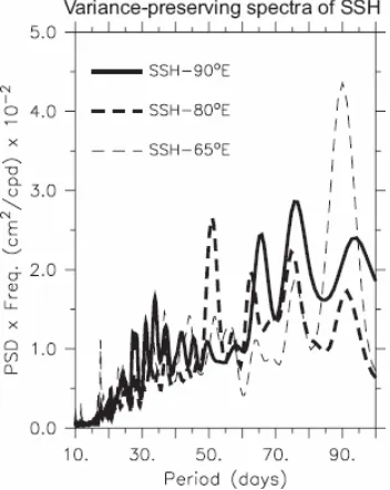
3.1 Spectral characteristics of intraseasonal sea levels Variance preserving spectra of sea level at three selected longitudes are shown in Figure 1. The spectra were calculated for the 200-month period November 1992 – June 2009. The spectra were estimated from the raw periodogram amplitudes by smoothing using triangle filter. The degree of freedom (DOF) was estimated according to the procedure of Bloomfield (1976), which results in 32 DOF.
The spectra given in Figure 1 show that a broad range of significant intraseasonal variability. Note that the longitudes chosen for Figure 1 are roughly at the maximum amplitudes of intraseasonal variability for SSH. There is an outstanding SSH variance at period of 90-day in the western basin. On the other hand, the spectra of the SSH observed in the central and eastern basin are more confined to higher frequency, though they still show energetic variance at period of 90-day. This 90-day variation has been clearly described in previous studies (Han, 2005; Fu, 2007) and will be excluded in our analysis.
Figure 1. Variance-preserving spectra of sea levels at 90°E (thick curve), 80°E (thick-dashed curve) and 65°E (thin-dashed curve). The spectra are calculated for the 200-month period November 1992 – June 2009.
3.2 Spatial structure of intraseasonal sea levels
To illustrate the basin-wide spatial and temporal structures of these intraseasonal signals, we apply CEOF analysis on the intraseasonal SSH over the region spanning 40°E – 100°E, 10°S – 10°N. Before applying a CEOF analysis, we performed a band-pass filter to the time series using wavelet filter (Torrence and Compo, 1998). As shown in the spectral analysis, the intraseasonal variations do not appear to have a fixed frequency band (Figure 1). We
selected the band of most energetic frequencies to define the intraseasonal variations in this study. The resulting band includes periods between 30 and 75 day. Thus, we apply 30–75-day band-pass filter to all quantities. Unless otherwise specified, all intraseasonal variabilities discussed in later sections are obtained in this manner.
It turns out that the leading CEOF mode represents 15.2% of the total SSH variability and the sum of the first four modes account for 34.8%. After evaluating the spatial structure of the first four CEOF modes, we found that only the first mode is closely resemble the structure of equatorial waves (e.g. Kelvin and Rossby waves). Thus, only this leading CEOF mode will be discussed hereafter.
The spatial amplitude and phase patterns of the leading mode are presented in Figure 2. The spatial amplitude structure (Figure 2a) contains two centers of activity; one along the equator from about 60°E extending eastward to the coast of Sumatra, and the other in the off equatorial region centered around 5°S and 5°N. The regions of high variability are concentrated in the eastern half of the basin roughly from 70°E extending eastward to the coast of Sumatra. Note that the large variability off Sumatra revealed in both CEOF modes is generated by the incoming Kelvin waves and their reflections at the eastern boundary.
The spatial phase pattern of the leading CEOF mode (Figure 2b) indicates an eastward propagation along the equator, while in the off equatorial region it indicates a westward propagation. This typical feature confirms the existence of Kelvin waves along the equator and Rossby waves off equator.
Figure 2. Spatial (a) amplitude (arbitrary unit), and (b) phase functions of the intraseasonal SSH obtained from the first mode of CEOF analysis.
3.3 Dynamics of intraseasonal sea levels
signals. Consider the distance between those two sites and the period of interest (e.g. 30 – 75 day), we obtained an estimated phase speed of 2.95 ± 1.77 m s-1. The estimated phase speed does not correspond to one particular baroclinic mode, though they fall within the range expected for the first three baroclinic modes (e.g. c1=2.5 m s-1, c2=1.55 m s-1, and c3=0.99
m s-1) in the equatorial Indian Ocean (Nagura and McPhaden, 2010).
Another method to estimate the phase speed is by fitting the meridional structure of the intraseasonal SSH to a Gaussian shape in the form of:
) 2 / exp( y2 λ2n
η= − , (8)
where y is latitude and λn =(cn/β)1/2 indicates the equatorial Rossby radius of deformation. Here, cn is
the phase speed of n-th baroclinic Kelvin wave, and β = 2.3 × 10⁻¹¹
m-1 s-1. We fit this Gaussian shape to the spatial pattern of the first CEOF mode at every 2° interval in longitude between 70°E and 96°E (Figure 3). The calculation results in an estimated phase speed of 1.99 ± 0.46 m s-1
, which again does not correspond exactly to a particular characteristic speed of baroclinic mode in the equatorial Indian Ocean obtained from the observation (Nagura and McPhaden, 2010). These results may suggest that the eastward propagating signals do not involve a single mode, instead they may contain the first and second (or even higher) baroclinic modes as previously suggested (Han, 2005; Fu, 2007; Iskandar et al., 2008).
Figure 3. Meridional sections of amplitude of the first CEOF mode (thick curve) and theoretical structure of Kelvin wave (thin-dashed curve) across (a) 76°E, (b) 80°E and (c) 90°E. The best-fit of phase speed at a given longitude is shown in each panel.
4. Summary and Discussion
This study examined the basin-wide structures of the intraseasonal sea level variations in the equatorial Indian Ocean using CEOF analysis. The spectra of sea levels indicate that within the intraseasonal time-scale, the variability is mostly confined within 30–75-day oscillation (Figure 1).
The spatial amplitude structure inferred from the CEOF analysis demonstrates that basin-wide structure of the intraseasonal sea levels resembles that of typical equatorial Kelvin and off-equatorial Rossby waves (Figure 2a). In addition, the spatial phase structures of the mode indicate an eastward propagation along the equator and a westward propagation in the off equatorial region (Figure 2b). These features may suggest that Kelvin waves play a role along the equator, while in the off equatorial region Rossby waves dominate the variability.
A calculation on phase difference along the equator from the first CEOF mode structure reveals an eastward propagation with phase speed of 2.95 ± 1.77 m s-1. This estimated phase speed falls within the range expected for the first three baroclinic modes in the equatorial Indian Ocean (Nagura and McPhaden, 2010). In addition, the phase speed of these propagating band-pass filtered signals can be estimated by fitting the spatial amplitude structures of the first CEOF mode to the theoretical Kelvin wave
structures (Figure 3). The phase speed estimated using this method is 1.99 ± 0.46 m s-1
, which again does not correspond exactly to a particular characteristic speed of baroclinic mode in the equatorial Indian Ocean (Nagura and McPhaden, 2010). These results suggest that the propagating signals do not involve a single baroclinic mode, but instead the first, second and possibly higher baroclinic modes. These results are consistent with the linear inviscid ray theory, which suggests that a superposition of several vertical modes is required for Kelvin wave energy to propagate as a beam of energy into the ocean interior (McCreary, 1984).
apparently observed in the deeper layer of the eastern basin.
Recent study on the seasonal cycle along the equatorial Indian Ocean has demonstrated that Rossby wave plays dominant role on the zonal current variations in the upper layer (Nagura and McPhaden, 2010). On the other hand, Kelvin and Rossby waves have comparable contributions on the SSH variations along the equator. In this study, we may expect a westward propagating signal along the equator if Rossby wave plays a role. Indeed, the band-pass filtered SSH and the reconstructed SSH from the first CEOF mode along the equator do not show such signal.
Acknowledgment
The author thanks Dr. Motoki Nagura of JAMSTEC for a fruitful discussion. The author also acknowledges the AVISO for providing gridded SSH dataset. The wavelet-filter was provided by C. Torrence and G. Compo and is available at
http://paos.colorado.edu/research/wavelets. This research was supported by the Directorate General of Higher Education (DGHE), Department of National Education, Indonesia.
References
Bloomfield, P., 1976, Fourier Decomposition of Time Series: An Introduction, 258 pp., John Wiley, New York.
Fu, L. L., 2007, Intraseasonal variability of the equatorial Indian Ocean observed from sea surface height, wind, and temperature data, J. Phys. Oceanogr., 37, 188-202.
Han, W., and J. P. McCreary, 2001, Modeling salinity distributions in the Indian Ocean, J. Geophys. Res., 106, 859–877.
Han, W., 2005, Origins and dynamics of the 90-day and 30-60 day variations in the equatorial Indian Ocean. J. Phys. Oceanogr., 35, 708-728.
Horel, J. D., 1984, Complex principal component analysis: theory and examples. J. Climate Appl. Meteor., 23,1660–1673.
Iskandar, I., T. Tozuka, Y. Masumoto and T. Yamagata, 2008, Impact of the Indian Ocean Dipole on intraseasonal zonal current at 90°E on the equator as revealed by self-organizing map, Geophys. Res. Lett. 35, L14S03, doi:10.1029/2008GL033468. Iskandar, I., and M. J. McPhaden, 2010, Dynamics of
wind-forced intraseasonal zonal current variations in the equatorial Indian Ocean, J. Geophys. Res., (in press).
Madden, R. A. and P. R. Julian, 1971, Detection of a 40−50 day oscillation in the zonal wind in the tropical Pacific, J. Atmos. Sci., 28, 702-708.
McCreary, J. P., 1984, Equatorial beams, J. Mar. Res., 42, 395–430.
McPhaden, M. J., 1982, Variability in the central equatorial Indian Ocean. Part I: Ocean dynamics, J. Mar. Res., 40, 157-176.
Nagura, M., and M. J. McPhaden, 2010, Wyrtki Jet dynamics: Seasonal variability, J. Geophys. Res., 115, C07009, doi: 10.1029/ 2009JC005922.