58 CHAPTER IV
RESULT OF THE STUDY
A. The Data Description
In this section, it described the obtained data of improvement the students’writing
recount text before and after taught by Cartoon Story maker and non-Cartoon Story
Maker. The presented data consisted of distribution of pre-test score of experimental and
control group and also the distribution of post-test score of experimental group and
control group.
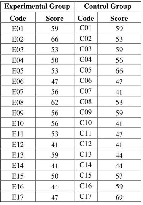
1. The Result of Pretest Score Experimental Group and Control Group Table 4.1 Pre-Test Score of Control and Experimental Group
Experimental Group Control Group Code Score Code Score
E01 59 C01 59
E02 66 C02 53
E03 53 C03 59
E04 50 C04 56
E05 53 C05 66
E06 47 C06 47
E07 56 C07 41
E08 62 C08 53
E09 56 C09 59
E10 56 C10 41
E11 53 C11 47
E12 41 C12 41
E13 59 C13 44
E14 41 C14 44
E15 50 C15 53
E16 44 C16 59
E18 56 C18 50
E19 47 C19 59
E20 41 C20 50
E21 53 C21 50
E22 53 C22 53
E23 53 C23 53
E24 59 C4 56
E25 47 C25 53
E26 59 C26 59
E27 53 C27 53
E28 50 C28 59
E29 56 C29 47
E30 66 30 53
E31 41 C31 47
E32 59 32 47
E33 53 C33 50
C34 56
C35 53
C36 56
a. The Result of Pretest Score of Experimental Group
The pre-test was conducted on Thursday, 11th August 2016 in the X-A
room. The students asked to write Recount text that interested them about the holiday
that should cover the generic structure consisted of identification and allocated time
was 90 minutes. The students’ pre-test score of experiment group were distributed in
the following table (see appendix 5) in order analyzing the students’ background
knowledge of Recount text before the treatment. Then, it was presented using
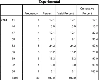
Table 4.2 Frequency Distribution of Pre-test Experiment Group
Experimental
Frequency Percent Valid Percent
Cumulative
Percent
Valid 41 4 12.1 12.1 12.1
44 1 3.0 3.0 15.2
47 4 12.1 12.1 27.3
50 3 9.1 9.1 36.4
53 8 24.2 24.2 60.6
56 5 15.2 15.2 75.8
59 5 15.2 15.2 90.9
62 1 3.0 3.0 93.9
66 2 6.1 6.1 100.0
Total 33 100.0 100.0
The distribution of students’ score in pre-test of the experimental group can
also be seen in the following figure.
Figure 4.1
The Distribution of Pre-Test Experimental Group
0 1 2 3 4 5 6 7 8 9
41 44 47 50 53 56 59 62 66
Based on the figure above, it can be seen that the students pretest score of
experiment group. There were four students who got score 41. There was one
student who got score 44. There were four students who got score 47. There were
three students who got score 50 . There were eight students who got score 53. There
were five students who got score 56. There was five students who got score 59. The
was one student who got score 62 and the last there were two students who got score
66.
The next step, the writer calculated the scores of mean, standard deviation,
and standard error using SPSS 21 program as follows.
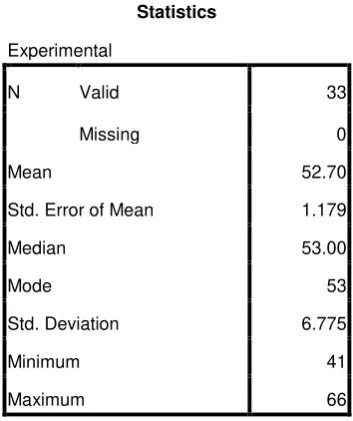
Table 4.3 The Calculation of Mean, Standard Error of Mean, Standard Deviation
Statistics
Experimental
N Valid 33
Missing 0
Mean 52.70
Std. Error of Mean 1.179
Median 53.00
Mode 53
Std. Deviation 6.775
Minimum 41
Maximum 66
Based on the calculation above, the higher score pre-test of the
experimental group was 66 and the lowest score was 41. And the result of the mean
was 52.70 median was 53.00, the mode was 53 the standard error of the mean was
b. The Result of Pretest Score of Control Group
The pre-test was conducted on Tuesday,23th August 2016 in the X-B room.
The students asked to write Recount text that interested them about the Holiday that
should cover the generic structure consisted of identification and allocated time was
90 minutes. The students’ pre-test score of the control group were distributed in the
following table (see appendix 5) in order analyzing the students’ background
knowledge. Then, it was presented using frequency distribution in the following table:
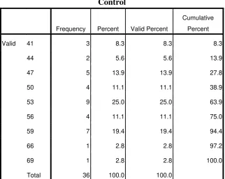
Table 4. 4 Frequency Distribution of Pre-test Control Group
Control
Frequency Percent Valid Percent
Cumulative
Percent
Valid 41 3 8.3 8.3 8.3
44 2 5.6 5.6 13.9
47 5 13.9 13.9 27.8
50 4 11.1 11.1 38.9
53 9 25.0 25.0 63.9
56 4 11.1 11.1 75.0
59 7 19.4 19.4 94.4
66 1 2.8 2.8 97.2
69 1 2.8 2.8 100.0
Total 36 100.0 100.0
The distribution of students’ score in pre-test of the experimental group can
Figure 4.2
The Distribution of Pre-Test Control Group
0 2 4 6 8 10
41 44 47 50 53 56 59 66 69
Frekuensi
Based on the figure above, it can be seen that the students pretest score of
the control group. There were three students who got score 41. There were two
students who got score 44. There were five students who got score 47. There were
four students who got score 50. There were nine students who got score 53. There
were four students who got score 56. There were seven students who got score 59.
There was one student who got score 66 and 69.
The next step, the writer calculated the scores of mean, standard deviation,
and standard error using SPSS 21 program as follows:
Table 4.5 The Calculation of Mean, Standard Error of Mean, Standard Deviation
Statistics
Control
N Valid 36
Missing 0
Mean 52.64
Std. Error of Mean 1.098
Median 53.00
Mode 53
Std. Deviation 6.586
Minimum 41
Based on the calculation above, the higher score pre-test of the control group
was 69 and the lowest score was 41. And the result of the mean was 52.64, the
median was 53,00, the mode was 53, the standard error of the mean was ,1.098 and
the standard deviation was 6.586.
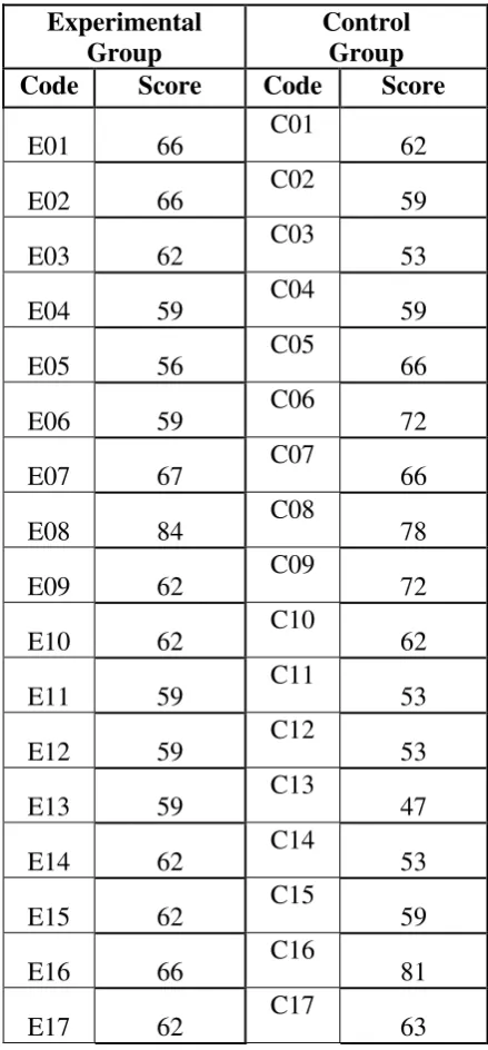
2. The Result of Post Test Score Experimental Group and Control Group Table 4.6 Post Test Score of Control and Experimental Group
Experimental Group
Control Group Code Score Code Score
E01 66 C01 62
E02 66 C02 59
E03 62 C03 53
E04 59 C04 59
E05 56 C05 66
E06 59 C06 72
E07 67 C07 66
E08 84 C08 78
E09 62 C09 72
E10 62 C10 62
E11 59 C11 53
E12 59 C12 53
E13 59 C13 47
E14 62 C14 53
E15 62 C15 59
E16 66 C16 81
E18 66 C18 52
E19 78 C19 66
E20 56 C20 53
E21 67 C21 66
E22 81 C22 53
E23 67 C23 62
E24 78 C24 59
E25 59 C25 56
E26 62 C26 66
E27 67 C27 53
E28 66 C28 66
E29 67 C29 69
E30 90 C30 69
E31 84 C31 69
E32 62 C32 69
E33 66 C33 66
C34
69 C35
59 C36
59
A.The Result of Post-test Score of Experimental Group
The post-test was conducted on Tuesday, 6th September 2016 in the X-A
room. The students asked to write recount text that interested them about the holiday
that should cover the generic structure consisted of identification, allocated time was
90 minutes and should post their text on Cartoon Story Maker. The students’
in order analyzing the students’ writing recount text after the treatment. Then, it was
presented using frequency distribution in the following table:
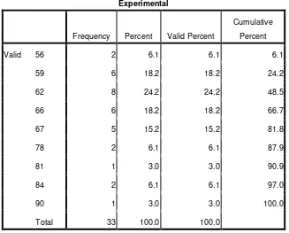
Table 4.7 Frequency Distribution of Post Test Experimental Group
Experimental
Frequency Percent Valid Percent
Cumulative
Percent
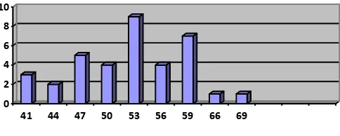
Valid 56 2 6.1 6.1 6.1
59 6 18.2 18.2 24.2
62 8 24.2 24.2 48.5
66 6 18.2 18.2 66.7
67 5 15.2 15.2 81.8
78 2 6.1 6.1 87.9
81 1 3.0 3.0 90.9
84 2 6.1 6.1 97.0
90 1 3.0 3.0 100.0
Total 33 100.0 100.0
The distribution of students’ score in pre-test of the Experimental group can
also be seen in the following figure.
Figure 4.3
The Distribution of Post Test Experimental Group
0 2 4 6 8
56 59 62 66 67 78 81 84 90
Based on the figure above, it can be seen that the students pretest score of
the control group. There were two students who got score 56. There were six
students who got score 59. There were eight students who got score 62. There were
six students who got score 66. There were five students who got score 67. There
were two students who got score 78. There were one student who got score 81.
There were two students who got score 84 and the last there was one student who
got score 90.
The next step, the writer calculated the scores of mean, standard deviation,
and standard error using SPSS 21 program as follow.
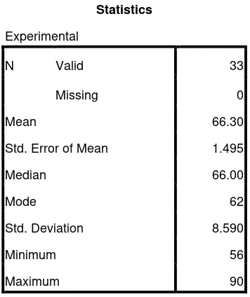
Table 4.8 The Calculation of Mean, Standard Error of Mean, Standard Deviation
Statistics
Experimental
N Valid 33
Missing 0
Mean 66.30
Std. Error of Mean 1.495
Median 66.00
Mode 62
Std. Deviation 8.590
Minimum 56
Maximum 90
Based on the calculation above, the higher score post test of the
experimental group was 90 and the lowest score was 56. And the result of the mean
was 66.30, the median was 66.00, the mode was 62, the standard error of mean was
B.The Result of Post-test Score of Control Group
The post-test was conducted on Wednesday 7th September 2016 in the X-B
room. The students asked to write recount text that interested them about the holiday
that should cover the generic structure consisted of identification, allocated time was
90 minutes The students’ post-test score of the control group were distributed in the
following table (see appendix 5) in order analyzing the knowledge of recount text.
Then, it was presented using frequency distribution in the following table:
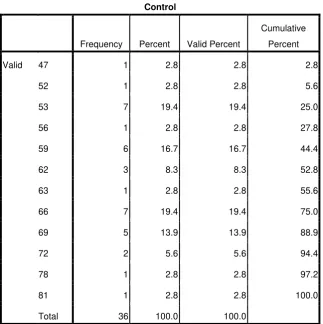
Table 4.9 Distribution Frequency of Post test Control Group
Control
Frequency Percent Valid Percent
Cumulative
Percent
Valid 47 1 2.8 2.8 2.8
52 1 2.8 2.8 5.6
53 7 19.4 19.4 25.0
56 1 2.8 2.8 27.8
59 6 16.7 16.7 44.4
62 3 8.3 8.3 52.8
63 1 2.8 2.8 55.6
66 7 19.4 19.4 75.0
69 5 13.9 13.9 88.9
72 2 5.6 5.6 94.4
78 1 2.8 2.8 97.2
81 1 2.8 2.8 100.0
Total 36 100.0 100.0
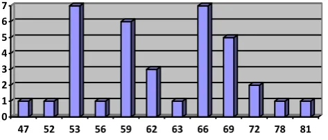
The distribution of students’ score in post test of control group could also
Figure 4. 4
The Distribution Frequency post-test Score for Control Group
0 1 2 3 4 5 6 7
47 52 53 56 59 62 63 66 69 72 78 81
Frekuensi
Figure 4.4 The Frequency of Distribution of Post test Control Group
Based on the figure above, it can be seen that the students post-test control
group. There was one student who got score 47. There was one student who got
score 52. There were seven students who got score 53. There was one student who
got score 56. There were six students who got score 59. There were three students
who got score 62. There was one student who got score 63. There were seven
students who got score 66. There were five students who got score 69. There were
two students who got score 72. There was one student who got score 78. And the last
there was one student who got score 81.
The next step, the writer calculated the scores of mean, standard deviation,
Table 4.10 The Manual Calculation of Mean, Standard Error of Mean, Standard Deviation
Statistics
Control
N Valid 36
Missing 0
Mean 62.19
Std. Error of Mean 1.308
Median 62.00
Mode 53
Std. Deviation 7.848
Minimum 47
Maximum 81
Based on the calculation above, the higher score pre-test of the control group
was 81 and the lowest score was 47. And the result of the mean was 62.19, the
median was 62.00, the mode was 53, the standard error of the mean was 1.308 and the
3. The Comparison Result of Pre-test and Post-test of Experimental and Control Group
Table 4.11 The Comparison Result of Pre-test and Post-test of Experimental and Control Group Experimental Control
No Code
Pre Test
Post
Test Improvement Code
Pre Test
Post
Test Improvement
1 E01 59 66 7 C01 59 62 3
2 E02 66 66 0 C02 53 59 6
3 E03 53 62 9 C03 59 53 -6
4 E04 50 59 9 C04 56 59 3
5 E05 53 56 3 C05 66 66 0
6 E06 47 59 12 C06 47 72 25
7 E07 56 67 11 C07 41 66 25
8 E08 62 84 22 C08 53 78 25
9 E09 56 62 6 C09 59 72 13
10 E10 56 62 6 C10 41 62 21
11 E11 53 59 6 C11 47 53 6
12 E12 41 59 18 C12 41 53 12
13 E13 59 59 0 C13 44 47 3
14 E14 41 62 21 C14 44 53 9
15 E15 50 62 10 C15 53 59 6
16 E16 44 66 22 C16 59 81 22
17 E17 47 62 15 C17 69 63 -6
18 E18 56 66 10 C18 50 52 2
19 E19 47 78 31 C19 59 66 7
20 E20 41 56 15 C20 50 53 3
21 E21 53 67 14 C21 50 66 16
22 E22 53 81 28 C22 53 53 0
23 E23 53 67 14 C23 53 62 9
24 E24 59 78 19 C24 56 59 3
25 E25 47 59 12 C25 53 56 3
26 E26 59 62 3 C26 59 66 7
28 E28 50 66 16 C28 59 66 7
29 E29 56 67 11 C29 47 69 22
30 E30 66 90 24 C30 53 69 16
31 E31 41 84 43 C31 47 69 22
32 E32 59 62 9 C32 47 69 22
33 E33 53 66 13 C33 50 66 16
34 E34 C34 56 69 13
35 E35 C35 53 59 6
36 E36 C36 56 59 3
Total 1739 2188 449 Total 1895 2239 344
Mean 52.70 66.30 Mean 52.64 62.19
Highest 41 56 Highest 41 47
Lowest 66 90 Lowest 69 81
B. Testing the Normality and Homogeneity 1. Normality Test
The writer used SPSS 21 to measure the normality of the data.
a) Testing Normality of Post Test Experimental and Control Group Table 4.12 Testing Normality of Post Test Experimental and Control
Group
One-Sample Kolmogorov-Smirnov Test
Experiment Control
N 33 36
Normal Parameters Mean 66.30 62.19
Std. Deviation 8.590 7.848
Most Extreme Differences Absolute .286 .131
Positive .286 .129
Negative -.137 -.131
Kolmogorov-Smirnov Z 1.642 .783
Asymp. Sig. (2-tailed) .009 .571
The criteria of the normality test of post-test if the value of (probability
value/critical value) was higher than or equal to the level of significance alpha
defined, it means that the distribution was normal. Based on the calculation used
SPSS 21.00 program, asymptotic significance normality of control group was
0.009 and experiment group 0.571 Then the normality both of class was
consulted with a table of Kolmogorov- Smirnov with the level of significance
5% (α=0.05). because asymptotic significance of control 0.571 > 0.05, and
asymptotic significance of experiment 0.009 > 0.05. it could be concluded that
the data was a normal distribution. It meant that the students’ pre-test score of
experimental and control group had a normal distribution.
2. Homogeneity Test
a). Testing Homogeneity of Post Test Experimental and Control Group Table 4.13 Testing Homogeneity of Post-Test Experimental and Control
Group
Test of Homogeneity of Variances
Experiment
Levene Statistic df1 df2 Sig.
2.127 5 21 .102
The criteria of the homogeneity test post test were if the value of
(probability value/critical value) was higher than or equal to the level of
significance alpha defined (r = a), it means that the distribution was homogeneity.
Based on the calculation using SPSS 21.0 above, the value of (probably
Homogeneity of Variances in sig column is known that p-value was 0,102. The
data in this study fulfilled homogeneity since the p-value is higher 0,102 > 0.05.
C. Result Data Analysis
1.Testing Hypothesis Using Manual Calculation
To test the hypothesis of the study, the writer used t-test statistical
calculation. Firstly, the writer calculated the standard deviation and the error of
X1 and X2 at the previous data presentation. In could be seen on this following
table:
Table 4.14
The Standard Deviation and Standard Error of X1 and X2
Variable The Standard Deviation
The Standard Error of Mean
X1 1. 495 8.590
X2 1.308 7.848
X1 = Experimental Group
X2 = Control Group
The table showed the result of the standard deviation calculation of X1 was 1.
495 and the result of the standard error mean calculation were 8.590. The result of the
standard deviation calculation of X2 was 1.308 and the result of the standard error mean
calculation was 7.848.
The next step, the writer calculated the standard error of the difference mean
Standard error of mean of score difference between Variable I and Variable II
SEM1– SEM2 = SEM12 + SEM22
SEM1– SEM2 =
SEM1– SEM2 =
SEM1– SEM2 = 2
SEM1– SEM2 = 1.163525676553
SEM1– SEM2 = 1.163
The calculation above showed the standard error of the differences mean
between X1 and X2 was 1.946. Then, it was inserted into the ttest formula to get the value
of t test as follows:
to =
to=
to =
to = 3.53
Which the criteria:
If t-test ≥ t-table, Ha is accepted and Ho is rejected
Then, the writer interpreted the result of t-test; previously, the writer accounted
the degree of freedom (df) with the formula:
Df = (N1+N2) -2
= 33+36 – 2 = 67
The resecher chose the significant levels at 5%, it means the significant level
of the refusal of null hypothesis at 5%. The researcher decided the significance level at
5% due to the hypothesis typed stated on non-directional (two-tailed test). It meant that
the hypothesis can’t direct the prediction of the alternative hypothesis. Alternative
hypothesis symbolized by “1”. This symbol could direct the answer of hypothesis, “1”
can be (>) or (<). The answer of hypothesis could not be predicted whether on more
than or less than.
The calculation above showed the result of t-test calculation as in the table
follows:
Table 4.15
The Result of T-Test Using Manual Calculation
Variable T-test T table Df/db
5 % 1 %
X1-X2 3.53 2.00 2.65 67
Where:
X1 = Experimental Group
T test = The Calculated Value
T table = The Distribution of t Value
Df/db = Degree of Freedom
Based on the result of hypothesis test calculation, it was found that the value of
observed was greater than the value of table at 1% and 5% significance level or 2.00< 3.53
>2.65. It means Ha was accepted and Ho was rejected. It meant Ha was accepted and Ho
was rejected. It could be interpreted based on the result of calculation that Ha stating that
Cartoon Story Maker was effective for Teaching Writing Recount Text of the tenth
grade students at MAN Katingan Hilir was accepted and Ho stating that Cartoon Story
Maker was not effective for Teaching Writing Recount Text of the tenth grade
students at MAN Katingan Hilir was rejected. It meant that teaching writing with
Cartoon Story Maker was effective for Teaching Writing Recount Text of the tenth
graders of MAN Katingan Hilir gave significant effect at 5% and 1% significance level.
2. Testing Hypothesis Using SPSS 21.0 Program
The researcher also applied SPSS 21.0 program to calculate t test in the testing
hypothesis of the study. The result of the t test using SPSS 21.0 was used to support the
manual calculation of the t test. The result of the test using SPSS 21.0 program could be
Table 4.16
Mean, Standard Deviation and Standard Error of Experiment Group and Control Group using SPSS 21.0 Program
Statistics
Experiment Control
N Valid 33 36
Missing 3 0
Mean 66.30 62.19
Std. Error of Mean 1.495 1.308
Std. Deviation 8.590 7.848
The table showed the result of mean calculation of experimental group was 66.30,
standard deviation calculation was 8.590, and standard error of mean calculation was 1.
495. The result of mean calculation of control group was 62.19., standard deviation
calculation was 7.848, and standard error of the mean was 1.308.
Table 4.17 The Calculation of T – Test Using SPSS 21.0
Independent Samples Test
Levene's Test
for Equality of
Variances t-test for Equality of Means
F Sig. T df
Sig.
(2-tailed)
Mean
Difference
Std. Error
Difference
95% Confidence
Interval of the
Difference
Lower Upper
Score
Equal variances
assumed .068 .795 2.076 67 .042 4.10859 1.97872 .15904 8.05813
Equal variances
The table showed the result of t – test calculation using SPSS 21.0 program. To know
the variances score of data, the formula could be seen as follows:
If α =0.05 < Sig, Ho accepted and Ha rejected
If α = 0.05> Sig, Ha accepted and Ho rejected
Since the result of post-test between experimental and control group had
difference score of variance, it found that α = 0.05 was higher than Sig (2-tailed) or
(0.05>0.00) so that Ha was accepted and Ho was rejected . The result of ttest was 3.53,
mean difference between experimental and control group was 4.10859 and the standard
error difference between experimental and control group was 1.97872.
To examine the truth or the false of null hypothesis stating that the there is no
effect of Project-Based Learning using Cartoon Story Maker in writing recount text at
tenth graders of MAN Katingan Hilir. The result of t – test was interpreted on the result of
the degree of freedom to get the ttable. The result of the degree of freedom (df) was 67. The
following table was the result of observed and ttable from 67 df at 5% and 1% significance level.
Table 4.18
The Result of T-Test Using SPSS 21.0 Program
t-test
t-table
Df 5 % (0,05) 1 % (0,01)
The interpretation of the result of t-test using SPSS 21.0 program, it was found
the t observe was greater than the t table at 5% significance level or 2.00<3.53>2.65. It
means that Ha was accepted and Howas rejected.It could be interpreted based on the result of
calculation that Ha stating that Project-Based Learning using Cartoon Story Maker was
effective for Teaching Writing Recount Text of the tenth grade students at MAN
Katingan Hilir was accepted and Ho stating that Project-Based Learning using Cartoon
Story Maker was not effective for Teaching Writing Recount Text of the tenth grade
students at MAN Katingan Hilir was rejected. It meant that teaching writing with Cartoon
Story Maker was effective for Teaching Writing Recount Text of the tenth graders at
MAN Katingan Hilir gave significant effect at 5% and 1 % significance level.
D. Discussion
The result of the analysis showed that there was a significant effect of
Project-Based Learning using Cartoon Story Maker in writing Recount text at tenth graders of
MAN Katingan Hilir It can be seen from the means score between pre-test and post-test.
The mean score of post test reached a higher score than the mean score of Pre-test (X=
53.61 < Y=50.14). It indicated that the students’ score increased after conducting
treatment. In other words, the students writing Recount text taught by Project-Based
Learning using Cartoon Story Maker have better than those taught by non-Project Based
Learning using Cartoon Story Maker at the tenth graders of MAN Katingan Hilir. There
are some problem when the treatment in school the firs media, media is very important to
learning writing using cartoon story maker, becouse in laboratory computer definite for
the students, so when learning the students bring laptop in school. The second lack a
vocabulary, so when the treatment the teacher gave vocabulary in each meeting, the
In addition, after the data was calculated using the ttest formula using SPSS
21.00 program showed that the observed was 3.53. In addition, After the students have been
taught by Cartoon Story Maker, the writing score was higher than before implementing
it. This finding indicated that Project-Based Learning using Cartoon Story Maker was
effective.
In teaching learning process, taught writing Recount text by using Cartoon Story
Maker was a tool used by the writer to teach the students. It could be seen from the score
of students how the used of Cartoon Story Maker gave positive effects for students
writing Recount text. It meant that it has an important role in teaching learning process.
It was answered the problem of the study which “Is there any significant effect of
Cartoon Story Maker in writing Recount text at tenth graders of MAN Katingan Hilir?”.
Project-Based Learning using Cartoon Story Maker as means for language
learning effectively enhanced the writing Recount text at tenth graders of MAN Katingan
Hilir. The students writing Recount text was enhanced after the treatment when they
were given opportunities to use Cartoon Story Maker in the learning process. They wrote
better Recount text using more meaningful contents within a well-organized text in the
post-test.
The results supported the theory by Dare and Gar in Chapter II page 14, stated that
Cartoon Story Maker helped students increase own language learning in a fun and
motivating way.51 The students gave their attention to the material because the writer
used different media than usual. Using Cartoon Story Maker as a media in writing text
actively encourages a collaborative environment, increases motivation and the student's
51
participation. They could update the writing assignments on Cartoon Story Maker and
their friends commented on their writing.
Next results supported the theory by Tarantino and Graf in Chapter II page 15,
stated that integrating Cartoon Story Maker in the foreign language course had several
perceived that using Cartoon Story Maker seems to have a significant impact on
language learning. Such as the nature of the students and
students-to-instructor instructions is more multi-dimensional than a traditional writing assignment.52
In line with it, the writer gave the students the assignment of Recount text and asked
them to post their writing on Cartoon Story Maker not on paper so that the students had
enthusiasm on produce the text.
The result of t-test using SPSS 21.0 program, it was found the t test was greater
than the t table at 5% significance level or 2.00<3.53>2.65. It means that Ha was accepted
and Howas rejected.It could be interpreted based on the result of a calculation that Ha stating
that Cartoon Story Maker was effective for Teaching Writing Recount Text of the tenth
graders of MAN Katingan Hilir was accepted and Ho stating that Cartoon Story Maker
was not effective for teaching writing Recount text of the tenth graders of MAN
Katingan Hilir was rejected. It meant that teaching writing with Cartoon Story Maker was
effective for teaching writing recount text of the tenth graders of MAN Katingan Hilir.
52