Implanted Antennas in Medical Wireless Communications pdf pdf

(1)

(2)

All rights reserved. No part of this publication may be reproduced, stored in a retrieval system, or transmitted in any form or by any means—electronic, mechanical, photocopy, recording, or any other except for brief quotations in printed reviews, without the prior permission of the publisher.

Implanted Antennas in Medical Wireless Communications Yahya Rahmat-Samii and Jaehoon Kim

www.morganclaypool.com

1598290541 paper Rahmat-Samii/Kim 159829055X ebook Rahmat-Samii/Kim

DOI 10.2200/S00024ED1V01Y200605ANT001

A Publication in the Morgan & Claypool Publishers’ series SYNTHESIS LECTURES ON ANTENNAS

Lecture #1

Series Editor: Constantine A. Balanis

First Edition 10 9 8 7 6 5 4 3 2 1

(3)

Implanted Antennas in Medical

Wireless Communications

Yahya Rahmat-Samii and Jaehoon Kim Department of Electrical Engineering,

University of California at Los Angeles

SYNTHESIS LECTURES ON ANTENNAS #1

M

(4)

ABSTRACT

One of the main objectives of this lecture is to summarize the results of recent research activities of the authors on the subject of implanted antennas for medical wireless communication systems. It is anticipated that ever sophisticated medical devices will be implanted inside the human body for medical telemetry and telemedicine. To establish effective and efficient wireless links with these devices, it is pivotal to give special attention to the antenna designs that are required to be low profile, small, safe and cost effective. In this book, it is demonstrated how advanced electromagnetic numerical techniques can be utilized to design these antennas inside as realistic human body environment as possible. Also it is shown how simplified models can assist the initial designs of these antennas in an efficient manner.

KEYWORDS

(5)

v

C H A P T E R 1

Implanted Antennas for Wireless

Communications

1.1 INTRODUCTION

The demand to utilize radio frequency antennas inside/outside a human body has risen for biomedical applications [1–3]. Most of the research on antennas for medical applications has focused on producing hyperthermia for medical treatments and monitoring various physiological parameters [1]. Antennas used to elevate the temperature of cancer tissues are located inside or outside of the patient’s body, and the shapes of antennas used depend on their locations. For instance, waveguide or low-profile antennas are externally positioned, and monopole or dipole antennas transformed from a coaxial cable are designed for internal use [1]. In addition to medical therapy and diagnosis, telecommunications are regarded as important functions for implantable medical devices (pacemakers, defibrillators, etc.) which need to transmit diagnostic information [3]. In contrast to the number of research accomplishments related to hyperthermia, work on antennas used to build the communication links between implanted devices and exterior instrument for biotelemetry are not widely reported.

It is commonly recognized that modern wireless technology will play an important role in making telemedicine possible. In not a distant future, remote health-care monitoring by wireless networks will be a feasible treatment for patients who have chronic disease (Parkinson or Alzheimer) [4]. To establish the required communication links for biomedical devices (wireless electrocardiograph, pacemaker), radio frequency antennas that are placed inside/outside of a human body need to be electromagnetically characterized through numerical and experimental techniques.

(8)

as realistic human body environment as possible. Also it is shown how simplified models can assist the initial designs of these antennas in an efficient manner.

1.2 CHARACTERIZATION OF IMPLANTED ANTENNAS

Figure 1.1 shows the schematic diagram of the research activities for implanted antennas in-side a human body for wireless communication applications. Implanted antennas are located inside a human head and a human body and are characterized using two different numerical

Measurement - Tissue-simulating fluid

Planar antenna Wire antenna

Analytical solution

Green’s function - Eigen-function

expansions - Simple geometries

FDTD

Maxwell equations - Complex geometries

In human body In human head

Implanted antennas in medical wireless communications

Numerical solution

- Differential

(9)

IMPLANTED ANTENNAS FOR WIRELESS COMMUNICATIONS 3

methodologies (spherical dyadic Green’s function (DGF) and finite difference time domain (FDTD)). There are clearly other numerical techniques that can be used. If an antenna is po-sitioned in a human head, the characteristic data for the antenna is obtained using spherical DGF expansions because the human head can be simplified as a lossy multi-layered sphere. This simplification provides useful capability to perform parametric studies. Numerical methodolo-gies (spherical DGF and FDTD) are implemented to characterize antennas inside a human head/body and to design implanted low-profile antennas to establish medical communication links between active medical implantable devices and exterior equipment.

For medical wireless communication applications, implanted antennas operate at the medical implant communications service (MICS) frequency band (402–405 MHz) which is regulated by the Federal Communication Commission (FCC) [5] and the European Radio-communications Committee (ERC) for ultra low power active medical implants [6].

1.2.1 Antennas Inside Biological Tissues

For implantable communication links between implanted antennas inside a human body and exterior antennas in free space, implanted antennas are located in biological tissues in two ways. As shown in Fig. 1.2, one way is that an implanted antenna directly contacts a biological tissue and the other is that an antenna indirectly contacts a biological tissue using a buffer layer. The buffer layer of Fig. 1.2(b) can be an air region or a dielectric material. The antenna of Fig. 1.2(a) requires smaller space in a human body than that of Fig. 1.2(b), but the link of Fig. 1.2(a) generates higher SAR value because of the direct contact. The advantage of Fig. 1.2(b) link is

Biological tissue

Buffer

(a) Directly contacting the biological tissue. (b) Indirectly contacting the biological tissue.

(10)

that there exist many possible methods to improve the performance of the communication link through diverse electrical characterization as it will be shown later.

1.2.2 Spherical Dyadic Green’s Function

For the spherical dyadic Green’s Function (DGF) simulations, a human head is approximated as a multi-layered lossy sphere with material characteristics based on measured data [7]. The expressions for the field distributions of the antenna inside the inhomogeneous sphere are obtained using the spherical DGF [8, 9]. By applying the infinitesimal current decomposition of the implanted antenna [10, 11] and introducing rotation of the coordinate system, the general expressions of the spherical DGF are modified to construct the required numerical codes. The law of energy conservation and the comparison of the results with the finite difference time domain (FDTD) simulations are used to verify the accuracy of the spherical DGF code.

1.2.3 Finite Difference Time Domain

For the FDTD analysis, the phantom data for a human body produced by computer tomography (CT) and the electric characteristic data of human biological tissues are combined to represent the input file for the computer simulations. The near-field distributions calculated from the spherical DGF code are compared with those from the FDTD code in order to evaluate the viability of the spherical DGF methodology for the analysis of implanted antennas inside a human head. To check how the human body affects the radiation characteristics of an implanted dipole in a human head, a three-dimensional geometry for the FDTD simulations was also constructed to include a human shoulder.

Beside characterization of wire antennas inside a human head or body, FDTD simulations are used to design planar antennas implanted inside a human body because of versatility of the FDTD code.

1.2.4 Design and Performance Evaluations of Planar Antennas

Based on the expected location of such implantable medical devices as pacemakers and car-dioverter defibrillators [12], low-profile antennas with high dielectric superstrate layers are designed under the skin tissues of the left upper chest area using FDTD simulations. Two antennas (spiral-type microstrip antenna and planar inverted F antenna) are tuned to a 50 system in order to operate at the MICS frequency band (402–405 MHz) for short-range med-ical devices. When the low-profile antennas are located in an anatomic human body model, their electrical characteristics are analyzed in terms of near-field and far-field patterns.

(11)

IMPLANTED ANTENNAS FOR WIRELESS COMMUNICATIONS 5

characteristics of the constructed implanted antennas to a 50system, the constructed antennas are inserted inside a tissue-simulating fluid whose electrical characteristics are very similar to those of the biological tissues. Maximum available power is calculated to analyze the reliability of the communication link and is used to estimate the minimum sensitivity requirement for receiving systems.

(12)

(13)

7

C H A P T E R 2

Computational Methods

In this chapter, the numerical methodologies discussed before (Green’s function and finite difference time domain (FDTD)) are utilized to characterize the antennas implanted inside a human body. To analyze the antennas in a human head, spherical Green’s functions are expressed in terms of spherical vector wave functions in order to obtain the closed form analytical formula. In addition, the input file for FDTD simulations which utilizes the integral form of Maxwell equations is generated.

2.1 GREEN’S FUNCTION METHODOLOGY

When an antenna is positioned in a human head, the characteristic data for the antenna is analytically obtained by simplifying the human head as a lossy multi-layered sphere. To facil-itate the numerical implementation of spherical Green’s function codes, infinitesimal current decomposition of the implanted source [10] and rotation of the coordinate system are utilized to modify the general spherical DGF expressions given in [9].

2.1.1 Spherical Head Models

A human head is represented as a multi-layered lossy dielectric sphere consisting of skin, fat, bone, dura, cerebrospinal fluid (CSF) and brain whose structure is shown in Fig. 2.1. Table 2.1 shows the electric characteristics (relative dielectric constant and conductivity) of the biological tissue in the model of the spherical head at 402 MHz using measured data from [8].

(14)

FIGURE 2.1: Schematic of the six-layered spherical head modeling a human head

TABLE 2.1: Electrical Characteristics of the Biological Tissues in the Spherical Head Models at 402 MHz

BIOLOGICAL TISSUE PERMITTIVITY (ε

r) CONDUCTIVITY (σ, S/m)

Brain 49.7 0.59

CSF 71.0 2.25

Dura 46.7 0.83

Skull 17.8 0.16

Fat 5.6 0.04

Skin 46.7 0.69

TABLE 2.2: Single-, Three- and Six-layered Spherical Head Models with an Outer Radius of 9 cm

BIOLOGICAL HOMOGENEOUS THREE-LAYERED SIX-LAYERED

TISSUE HEAD (cm) HEAD (cm) HEAD (cm)

Brain a1=9.00 a3=8.10 a6=8.10

CSF a5=8.30

Dura a4=8.35

Bone a2=8.55 a3=8.76

Fat a2=8.90

(15)

COMPUTATIONAL METHODS 9

2.1.2 Spherical Green Function’s Expansion

By modeling a human head as a sphere consisting of multiple layers of different lossy dielectric materials, the antenna implanted in a human head is represented as the current source in the multi-layered sphere as shown in Fig. 2.2. The total electric field,Ef in the field layer generated by current density of the implanted source, Js(r′) in the source layer can be calculated by the volume integration in terms of the spherical dyadic Green’s Functions (DGF) [8]:

Ef(r)= −jωμs

v

Ge0(r,r′)δf s +G

(f s) es (r,r

′ )

·Js(r′)d v′ (2.1)

where ω is the angular frequency, μ_s the permeability of the source layer, r =(r, θ , φ) the field location,r′ =(r0, θ0, φ0) the source location, andδf s the Kronecker delta. In addition,

Ge0(r,r′) is an unbounded spherical DGF in the source region, and G (f s) es (r,r

′_{) is a} scat-tering spherical DGF for the field in the field layer from the current source in the source

(16)

layer [9]: determined using the boundary conditions among the multi-layers, and Me(i)

omn,N (i) e

(17)

2.1.3 Simplification of Spherical Green’s Function Expansion

Two techniques are utilized to simplify the calculation of the Green’s function expansion in the form of Eq. (2.1). The first technique in reducing the complexity of the volume integration is to represent the dipole antenna as superposition of infinitesimal current elements lining up along the antenna [10, 11], as shown in Fig. 2.3. Furthermore, by rotating the coordinate system, one is able to decompose each current element into its localx1-directed andz1-directed components on the assumption that the dipole is positioned in the x–zplane [17]. In Fig. 2.3, Ilx(r_l′, 0, 0) and Ilz(rl′, 0, 0) represent the x-directed and z-directed current moments decomposed from the original current moment using the rotation of the coordinate system.

Based on the decomposition of the dipole antenna and the rotation of the coordinate system for each current element, the electric field expression based on the local (rotated) co-ordinate system (xl, yl,zl) from each infinitesimal current moment modified from Eq. (2.1) is given as:

x(rl) are the incident and scattering electric fields from an x-directed infinitesimal electric current moment on the z-axis. Simi-larly, Ei_z(rl) and E

s

z(rl) represent the incident and scattering electric fields from az-directed infinitesimal electric current moment on thez-axis.

(18)

Becausexdirection ( ˆxl) on thez-axis is equal to theθ direction ( ˆθl) in the local spher-ical coordinate system, the scattering electric field expression from anx-directed infinitesimal electric current moment on thez-axis is reformulated as:

E_xs (rl)= −jωμfIlxG spherical coordinate system, the scattering electric field from az-directed infinitesimal electric current on thez-axis is given as:

E_zs (rl)= −jωμfIlzG

To restore the actual electric field, the coordinate transformation is needed to return to the original coordinate system (x, y,z).

2.2 FINITE DIFFERENCE TIME DOMAIN METHODOLOGY

(19)

FIGURE 2.4: Schematic diagram for the FDTD input file (geometry) generation

2.2.1 Input File for FDTD Simulation

To simulate implanted antennas in a human body, the input file for FDTD codes needed to be prepared. The first step is to make an anatomical body model which is read by a FDTD computer code and the second is to locate implanted antennas inside the body model. Figure 2.4 shows how to translate the phantom data for a human body produced by raw computer tomography (CT) into the input file needed for the FDTD simulations. By using the tissue information, the proper electric characteristic data such as permittivity, conductivity, and mass density are assigned to each voxel. Antennas are properly located and operated inside a human head/body by applying specific information (the shape, location, input values) about implanted antennas. The electric and magnetic fields at every unit cell are updated by using the integral form of Maxwell equations.

2.2.2 Human Body Model

(20)

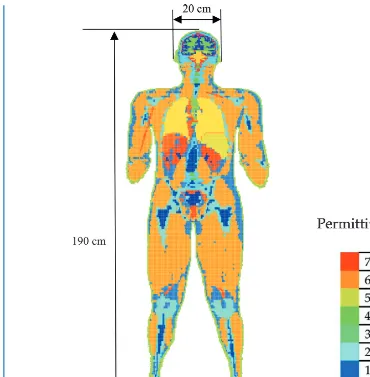
FIGURE 2.5: A human body model represented by different relative permittivity

the voxel size (4 mm) of the phantom file. According to Table 2.3, the range of the conductivity for biological tissues is from about 0 to 3 S/m, and the relative permeability for biological tissues is 1. The mass densities of biological tissues taken from [19] are between 0 and 2 g/cm3.

2.3 NUMERICAL TECHNIQUES VERIFICATIONS

BY COMPARISONS

(21)

TABLE 2.3: Electrical Data of Biological Tissues Used for the Human Body Model at 402 MHz

BIOLOGICAL PERMITTIVITY CONDUCTIVITY MASS DENSITY

TISSUE (ε

r) (σ, S/m) (g/cm

3₎

Brain 49.7 0.59 1.04

Cerebrospinal fluid 71.0 2.25 1.01

Dura 46.7 0.83 1.01

Bone 13.1 0.09 1.81

Fat 11.6 0.08 0.92

Skin 46.7 0.69 1.01

Skull 17.8 0.16 1.81

Spinal cord 35.4 0.45 1.04

Muscle 58.8 0.84 1.04

Blood 64.2 1.35 1.06

Bone marrow 5.67 0.03 1.06

Trachea 44.2 0.64 1.10

Cartilage 45.4 0.59 1.10

Jaw bone 22.4 0.23 1.85

Cerebellum 55.9 1.03 1.05

Tongue 57.7 0.77 1.05

Mouth cavity 1.0 0.00 0.00

Eye tissue 57.7 1.00 1.17

Lens 48.1 0.67 1.05

Teeth 22.4 0.23 1.85

Lungs 54.6 0.68 1.05

Heart 66.0 0.97 1.05

Liver 51.2 0.65 1.05

Kidney 66.4 1.10 1.05

Stomach 67.5 1.00 1.05

Colon 66.1 1.90 1.05

Thyroid 61.5 0.88 1.05

Trachea 44.2 0.64 1.10

Spleen 63.2 1.03 1.05

(22)

2.3.1 Comparison with the Closed Form Equation

Two electric field intensities are compared in Fig. 2.6. One is for an infinitesimal dipole placed in the free space and the other is for an infinitesimal dipole located at the center of a homogeneous lossless dielectric (ε_r =49.0,σ =0. S/m) sphere whose radius is 9 cm. All dipoles are assumed to deliver 1 W (watt) at 402 MHz. When the dipole is located in the free space, the electric field intensity along thez-axis is calculated by the following closed form equation [20]:

and Il the infinitesimal current moment which is determined by the following radiated power equation:

When the dipole is in the dielectric sphere, the electric field intensity along thez-axis is obtained by the spherical DGF code. The dipole placed inside the dielectric sphere produces a

radius = 9 cm

(23)

(24)

standing wave pattern which depends on the operating frequency. The important observation is that both electric field distributions outside the sphere are the same because power is not dissipated in the lossless environment.

2.3.2 Comparison with FDTD

In this section, the spherical DGF implementation is compared with the FDTD simulations using the same simulation structure. For this comparison, dipole antennas are normalized to deliver the same power. The spherical code uses Eq. (2.11) in order to control the delivered power. The delivered power,Pdelat the source point is divided into the incident power,Pincdelivered by the initial current and the scattered power,Pscagenerated by the interaction between the initial current and the surrounding environment. The incident power and the scattered power are expressed by volume integrations using an unbounded spherical DGF and a scattering spherical DGF expression. Finally, the total power is generated from the initial current density, Js of the dipole. Equation (2.9) shows that the total power delivered from antennas can be controlled by revising the initial current, Js:

Pdel(r =_r′)= _P_inc(r =_r′)+_Psca(r =_r′)= −1

For the FDTD code to control the delivered power, the fact that real delivered power is equal to the sum of the radiated power and the absorbed power in a lossy medium is applied.

(25)

19

C H A P T E R 3

Antennas Inside a Biological Tissue

3.1 SIMPLE WIRE ANTENNAS IN FREE SPACE

Simple wire antennas, dipoles and loops, in the free-space region are studied to examine field behaviors around the antennas before implanting them in biological tissues. The near-field distributions from the simple antennas in the free space are calculated in three ways: the theoretical expressions, finite difference time domain (FDTD) code, and method of moments (MoM) code to confirm the FDTD simulations which are applied to characterize the simple wire antennas inside a biological tissue.

3.1.1 Characterization of Dipole Antennas

Figure 3.1 shows a small dipole antenna located in the free space. The dipole antenna is 0.03 wavelength (λ) at 402 MHz in length and is oriented along the z-axis. The center of the coordinate system is located at the feeding point of the dipole antenna.

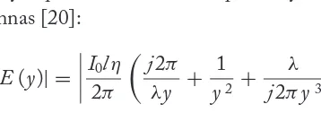
The electric and magnetic field magnitudes along they-axis for the small dipole in Fig. 3.1 are theoretically expressed by Eqs. (3.1) and (3.2), respectively, which are valid field equations for 0.02–0.1λ₀dipole antennas [20]:

|E(y)| =

whereI0is the maximum current of the small dipole,l the dipole’s length,ηthe wave impedance (=120π) in the free space andλthe wavelength. The maximum current is given in Eq. (3.3) and the radiation impedance, Rr, of the dipole is calculated in Eq. (3.4) [20]:

(26)

y

l = 0.03l at 402 MHz

z

x

FIGURE 3.1: Small dipole antenna in the free space

According to Eqs. (3.1) and (3.2), the near electric field around the dipole antenna is proportional to the inverse cube of the radial distance while the near magnetic field is propor-tional to the inverse square of the radial distance. It means that electric fields would be more advantageous than magnetic field when one couples the energy from electric field sources in the near-field region.

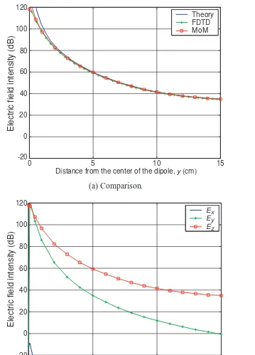
To examine the exact field value from the small dipole, the near-field distributions of the small dipole along y-axis are calculated in three ways: the theoretical expressions, finite difference time domain (FDTD) code, and method of moments (MoM) code. In Fig. 3.2, the electric field distributions from the dipole antenna are compared. The dipole radiates 1 W into the free space and its operating frequency is 402 MHz. Three total electric field distributions in Fig. 3.2(a) are very similar except around the dipole’s location which is known as a singular point. The theory generates higher electric field intensity than the real value around the singular point. By using the MoM code, Fig. 3.2(b) gives three electric field components decomposed from the total electric field. TheEx component is negligible along they-axis. The magnitude of the Eycomponent only near the dipole antenna is similar to that of theEzbecause circular electric field lines are generated between two polarities of the dipole. However, as the observation point extends far from the center of the dipole, the radial electric (Ey) component diminishes faster than the vertical electric field (Ez) component.

(27)

ANTENNAS INSIDE A BIOLOGICAL TISSUE 21

0 5 10 15

-20 0 20 40 60 80 100 120

Distance from the center of the dipole, y (cm) Theory FDTD MoM

(a) Comparison.

0 5 10 15

-20 0 20 40 60 80 100 120

Distance from the center of the dipole, y (cm) E_x E_y E_z

Electric field intensity (dB)

(b) Decomposition of total electric field using MoM.

(28)

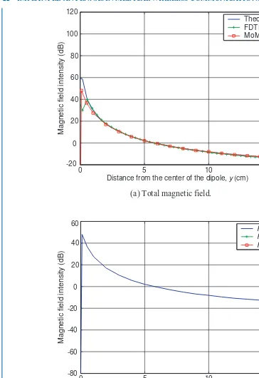
0 5 10 15 -20

0 20 40 60 80 100 120

Distance from the center of the dipole, y (cm) Theory FDTD MoM

(a) Total magnetic field.

0 5 10 15

-80 -60 -40 -20 0 20 40 60

Distance from the center of the dipole,y (cm) Hx

Hy

Hz

(b) Decomposition of total magnetic field using MoM.

Magnetic field intensity (dB)

(29)

almost the same as that of the total magnetic field and the other components are too small to be shown in Fig. 3.3(b). Therefore, only the horizontal electric field component exists along the y-axis.

From Figs. 3.2 and 3.3, the wave impedance can be obtained by dividing the total electric field by the total magnetic field component. At 5 cm from the center of the dipole, because the total electric field intensity is about 60 dB and the total magnetic field is about 2 dB, the wave impedance is 58 dB. If the wave impedance is calculated at nearer than 5 cm, the value is higher than 58 dB. Therefore, it is expected that the wave impedance near the small dipole is much higher than the intrinsic impedance (120π =51.5 dB) of a transverse electromagnetic (TEM) wave. It is observed that at 15 cm the wave impedance is similar to the intrinsic impedance of a TEM wave.

3.1.2 Characterization of Loop Antennas

Figure 3.4 shows a square loop antenna located in the free space. The square loop’s side-width (w) is 0.03 wavelength (λ₀) at 402 MHz and the total length (l) is 0.12λ₀. The origin of the coordinate system is located at the center of the loop antenna and the antenna is parallel to the x–zplane. The square loop is fed at the side of the loop, as shown in Fig. 3.4.

The magnetic field magnitude along they-axis of the loop antenna in Fig. 3.4 is obtained from Eq. (3.5) which is a valid theoretical expression for a small circular loop antenna [20]. Because the theoretical expression for a small circular loop antenna creates a null electric field magnitude along the y-axis, the expression for the electric field magnitude is omitted:

|H(y)| =

(30)

whereI0is the constant current of the small loop,Sthe loop’s area, andλthe wavelength. The constant current is given in Eq. (3.3) and the radiation impedance,Rr, of the loop is calculated in Eq. (3.6):

According to Eq. (3.5), the near magnetic field around a small loop antenna varies as the inverse cube of the radial distance, similarly to a small dipole antenna whose electric field varies as the inverse cube of the radial distance.

The near electric field distributions from the square loop antennas are calculated in Fig. 3.5. The loop antenna is fed to radiate 1 W into the free space at 402 MHz. Because of the theoretical null electric field along the y-axis, the theoretical calculation is not included in Fig. 3.5. The total electric field distributions along the y-axis are calculated by the FDTD and the method of moments (MOM) codes. It is found that two simulated electric field distri-butions are very similar to each other. From the MoM code, total electric field from the loop antenna is decomposed into the three electric field components (Ex, Ey, andEz), as shown in Fig. 3.5(b). As expected, thezelectric component (Ez) along they-axis is dominant and almost the same as the total magnetic field.

The near magnetic field distributions for the square loop obtained from the FDTD and MoM simulations are compared with those for a small circular loop from the theoretical expressions in Fig. 3.6. In Fig. 3.6(a), the total magnetic field from FDTD is well matched to the field from MOM although the theory generates higher field values near the antenna because the theoretical expression is for a small circular loop antenna. Therefore, it is expected that smaller loop antennas generate higher near magnetic fields. The decomposed magnetic fields are shown in Fig. 3.6(b). Because the longitudinal magnetic component, Hy along the y-axis is dominant, a receiving antenna should be properly located to maximize the power coupling from a transmitting loop antenna.

(31)

0 5 10 15

-20 0 20 40 60 80 100 120

Distance from the center of the loop, y (cm) FDTD MoM

(a) Total electric field.

0 5 10 15

-20 0 20 40 60 80 100 120

Distance from the center of the loop, y (cm) Ex

Ey

Ez

(b) Decomposition of total electric field using MoM.

(32)

0 5 10 15 -20

0 20 40 60 80 100 120

Distance from the center of the loop, y (cm) Theory FDTD MoM

(a) Total magnetic field.

0 5

Magnetic field intensity (dB)

10 15

-80 -60 -40 -20 0 20 40 60

Distance from the center of the loop, y (cm) Hx

Hy

Hz

(b) Decomposition of total magnetic field using MoM.

(33)

3.2 WIRE ANTENNAS IN BIOLOGICAL TISSUE

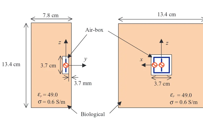
To characterize simple wire antennas inside a biological tissue by using FDTD simulations, the dipole antenna in Fig. 3.1 and the loop antenna in Fig. 3.4 are located in a simplified biological tissue whose dimensions are 13.4 cm ×7.8 cm × 13.4 cm, as shown in Fig. 3.7. The length (0.03λat 402 MHz=2.2 cm) of the dipole is the same as the side-width of the loop. The simplified body model is uniformly filled with a single biological tissue whose relative permittivity (ε_r) is 49, relative permeability (µ_r) 1, and conductivity (σ) 0.6 S/m.

The antennas implanted in the simplified model is centered at an air-box whose dimen-sions are 3.7 cm×0.7 cm×3.7 cm. Because it is assumed that the implanted antennas are located under a skin biological tissue in a human body, the depth (3.7 mm) of the air-box from the free space represents the thickness of the skin tissue. The center of the air-box is the same as the centers of the wire antennas.

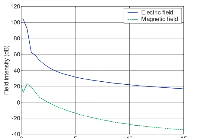
Figure 3.8 shows the electric and magnetic field distributions along the y-axis from the dipole antenna in the simplified tissue model. The antenna is assumed to deliver 1 W and operate at 402 MHz. At the boundary between the tissue and the free space, it is observed that the slope of the electric field is abruptly changed.

Table 3.1 shows the electric field and magnetic field variations along the radial direction (y-axis) from the dipole in the free space and the biological tissue. The field variations are

7.8 cm

(34)

0 5 10 15 -40

-20 0 20 40 60 80 100 120

Distance from the center of the dipole, y (cm) Electric field Magnetic field

Field intensity (dB)

FIGURE 3.8: Field distributions along they-axis from the small dipole in the biological tissue

observed at two locations, 5 and 15 cm away from the dipole. At 5 cm, the difference of the electric field between the free space and the biological tissue case is 28 dB while the difference of the magnetic field is 16 dB. It means that in the near-field region, the electric field intensity from the dipole in a biological tissue decreases faster than the magnetic field. At 15 cm, the difference of the electric field between in the free space and the biological tissue is 19 dB while the difference of the magnetic field is 20 dB. In the far-field region, the electric field intensity from the dipole in the tissue decreases similarly to the magnetic field. At 15 cm, the difference (48.8 dB) between the electric and magnetic field intensity from the dipole in the biological tissue approaches to the intrinsic impedance (51.5 dB).

TABLE 3.1: Electric Field (V/m) and Magnetic Field (A/m) Variations Between the Dipoles in the Free Space and in the Biological Tissue (Delivered Power=1 W)

5 cm 15 cm

OBSERVATIONS E_{(V/m dB)} H_{(A/m dB)} E_{(V/m dB)} H_{(A/m dB)}

Dipole in free space 59.2 2.2 34.7 −14.1

(35)

0 5 10 15

-40 -20 0 20 40 60 80 100 120

Distance from the center of the loop, y (cm) Electric field Magnetic field

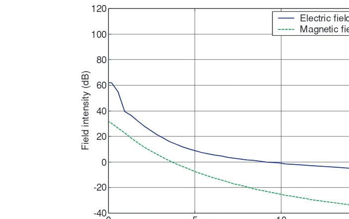
FIGURE 3.9: Field distributions along they-axis from a square loop antenna in the biological tissue

Figure 3.9 shows the electric and magnetic field distributions along the y-axis from the loop antenna in the simplified tissue model. At the boundary between the tissue and the free space, abrupt variation in the slope of the electric field is observed while the magnetic field decreases continuously along they-axis. The difference between the electric field and magnetic field increases as the distance increases from the antenna.

Table 3.2 shows the electric field and magnetic field variations along they-axis from the loop. Similarly to dipole antenna, the field variations are observed at two locations, 5 and 15 cm from the center of the loop. At 5 cm, the difference of the electric field between the free space and the biological tissue case is 36 dB while that of the magnetic field is 18 dB. The electric field from the loop in the biological tissue decreases faster than the magnetic field as the distance

TABLE 3.2: Electric Field (V/m) and Magnetic Field (A/m) Variations Between the Loops in the Free Space and in the Biological Tissue (Delivered Power=1 W)

5 cm 15 cm

Loop in free space 47.3 13.3 22.8 −10.7

(36)

increases. The fact that the wave impedance from the loop in the tissue model is 18.6 dB at 5 cm indicates that the longitudinal magnetic field (Hy along the y-axis) is very strong in front of the tissue model. At 15 cm, the difference of the electric field between the free space and the biological tissue case is 26 dB while the difference of the magnetic field is 24 dB. In the far-field region, the electric field intensity of the loop in the tissue decreases similarly to the magnetic field. Because the wave impedance from the loop in the tissue model is 32 dB at 15 cm, it is expected that the longitudinal magnetic component is still dominant at this distance.

3.3 EFFECTS OF CONDUCTOR ON SMALL WIRE ANTENNAS IN

BIOLOGICAL TISSUE

It is expected that implanted antennas are mounted on the conductive cases of active implantable medical devices in order to wirelessly communicate with the outside. The characteristic varia-tions of the simple antennas by a conductive plate are estimated only in terms of the near electric and magnetic field intensities. The effects of the metallic plate on the characteristics of simple wire antennas are analyzed by the FDTD simulations. The same simulation structures as shown in Fig. 3.7 are utilized to evaluate the variation of the field distributions from the small wire antennas.

As shown in Fig. 3.10, a conductive plate which is parallel to thex–yplane is additionally included in the simulation structure behind the small wire antennas. The conductive plate can be considered as the surface of implantable medical devices. The wire antenna’s input impedance

7.8 cm

(37)

0 5 10 15

-40 -20 0 20 40 60 80 100 120

Distance from the center of the dipole, y (cm) Electric field Magnetic field

FIGURE 3.11: Field distributions along they-axis from the small dipole in front of conductive plate in the biological tissue

is affected by the conductive plate. The impedance matching characteristic of the antenna is not considered here. The near-field variations from the dipole/loop antennas are the main focus in this chapter.

Figure 3.11 shows the electric and magnetic field distributions along they-axis from the dipole antenna in front of the conductive plate in the simplified tissue model of Fig. 3.10. The dipole antenna delivers 1 W. Because the field distributions of Fig. 3.11 are very similar to those of Fig. 3.8, a detailed comparison between the two cases is required (Table 3.3).

From Table 3.3, it is observed that the conductive plate affects the electric field intensities by a slight increase of 0.3 dB along the y-axis although no variation in the magnetic field intensity is observed.

TABLE 3.3: Variations of Electric Field (V/m) and Magnetic Field (A/m) from the Dipole in the Biological Tissue by the Conductive Plate (Delivered Power=1 W)

5 cm 15 cm

Without metal plate 31.2 −13.6 16.5 −34.5

(38)

0 5 10 15 -40

-20 0 20 40 60 80 100 120

Distance from the center of the loop, y (cm) Electric field Magnetic field

FIGURE 3.12: Field distributions along they-axis from the small loop in front of conductive plate in the biological tissue

The electric and magnetic field distributions along they-axis from the loop antenna in front of the conductive plate in the simplified tissue model are calculated in Fig. 3.12. The loop antenna delivers 1 W. The field distributions of Fig. 3.12 are very similar to those of Fig. 3.9 and a detailed comparison between the two cases is given in Table 3.4.

From Table 3.4, the electric field intensities vary from 11.3 to 8.9 dB (V/m) at 5 cm and from−3.1 to−5.5 dB (V/m) at 15 cm because of the metallic plate. The decreased values are the same as 2.4 dB at 5 and 15 cm. The fact that the magnetic field intensities are not changed signifies that the receiving power is not changed if the magnetic field from a loop antenna is coupled in the near-field region at the outside.

TABLE 3.4: Variations of Electric Field (V/m) and Magnetic Field (A/m) from the Loop in the Biological Tissue by the Conductive Plate (Delivered Power=1 W)

5 cm 15 cm

Without metal plate 11.3 −7.3 −3.1 −35.1

(39)

33

C H A P T E R 4

Antennas Inside a Human Head

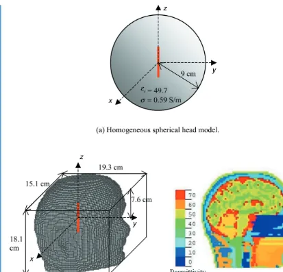
To ensure that applying simplified spherical head models for the characterization of implanted antennas in a head is adequate, electric field distributions from a dipole antenna in the spherical head model are compared with those in an anatomical head model. Three types of the spherical head models are used to assess how much the performance of implanted antennas depends on the head configurations. Based on the results of the dependency estimation, the maximum available power is calculated to give basic insights about the performance of the biomedical links built by implanted antennas in the spherical adult’s and child’s heads.

4.1 APPLICABILITY OF THE SPHERICAL HEAD MODELS

To reduce the discrepancies and increase the usefulness of the simplified spherical head models for the implanted antennas’ characterization, the volume of the spherical head model should be matched to that of the anatomical head model. For the volume matching, the anatomical head model was scaled down from the original human phantom file of Fig. 2.5 in order to make the anatomical head’s volume equal to the homogeneous spherical head’s (radius=9 cm, volume=

3.05×10−3m3) as shown in Fig. 4.1. The spherical head model of Fig. 4.1(a) for the spherical

DGF simulations is composed of a single brain tissue. The anatomical head of Fig. 4.1(a) for the FDTD simulations consists of various biological tissues whose electrical characteristics are given in Table 4.1.

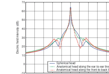
Figure 4.2 shows near electric field distributions calculated from the spherical DGF and FDTD codes. The dipole antennas (length = 5.3 cm) are positioned at the centers of the

(40)

FIGURE 4.1: Volume-matched spherical head and anatomical head models

The condition for utilizing the spherical head model is that the volume of the spherical model should be matched to that of the anatomical head model.

4.2 ANTENNAS IN VARIOUS SPHERICAL HEAD MODELS

(41)

ANTENNAS INSIDE A HUMAN HEAD 35

TABLE 4.1: Electrical Constants of Biological Tissues Used for the Anatomical Head Model at 402 MHz

BIOLOGICAL CONDUCTIVITY

TISSUE PERMITTIVITY (ε

r) (σ, S/m)

Brain 49.7 0.59

Cerebrospinal fluid 71.0 2.25

Dura 46.7 0.83

Bone 13.1 0.09

Fat 11.6 0.08

Skin 46.7 0.69

Skull 17.8 0.16

Muscle 58.8 0.84

Blood 64.2 1.35

Cartilage 45.4 0.59

Jaw bone 22.4 0.23

Cerebellum 55.9 1.03

Tongue 57.7 0.77

Mouth cavity 1.0 0.00

Eye tissue 57.7 1.00

Lens 48.1 0.67

Teeth 22.4 0.23

and 4.5 cm from the centers of the three kinds of heads (homogeneous, three-layered, and six-layered) as given in Table 2.2.

(42)

-25 -20 -15 -10 -5 0 5 10 15 20 25 -10

0 10 20 30 40 50 60 70

Radial distance, x, y (cm) Spherical head

Anatomical head along the ear-to-ear line Anatomical head along the front-to-back line

Electr

ic field intensity (dB)

FIGURE 4.2: Near-field distributions for dipole antennas implanted at the centers of the volume-matched spherical and anatomical head models

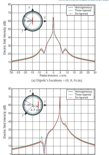
Radiated powers from the half-wavelength dipole in the spherical head models (radius=

9 cm) at 402 MHz are compared in Table 4.2 when the delivered power is 1 W. Although the radiated powers for the three-layered head case are higher than those for other cases when the dipoles are located at the centers of the head models and 4.5 cm away from the centers, the differences are very small.

TABLE 4.2: Radiated Power from the Dipole in the Various Spherical Head Models (Delivered Power=1 W)

HEAD DIPOLE (0, 0, 0 cm) DIPOLE (0, 0, 4.5 cm)

MODELS at 402 MHz at 402 MHz

Homogeneous 14.7 mW 7.2 mW

Three-layered 16.6 mW 8.0 mW

(43)

(44)

As the near-field distributions and radiated power of the dipole antenna inside three kinds of the spherical head models are similar to each other, the co-polarized far-field patterns of the implanted dipole (length=5.3 cm) only in the homogeneous head are calculated at 402 MHz in

Fig. 4.4. The far-field patterns are normalized using the maximum radiation power. As shown in Fig. 4.4(a), when the dipole is located at the center of the head (0, 0, 0 cm), the horizontal and vertical patterns are very similar to those of the dipole in the free space. As shown in Fig. 4.4(b), when the dipole is moved away from the head center (0, 0, 4.5 cm), the patterns become distorted because of the asymmetry of the source location.

4.3 SHOULDER’S EFFECTS ON ANTENNAS IN A HUMAN HEAD

In the previous chapter, characteristic data for implanted antenna inside a head are generated without consideration of a human body. Therefore, it is necessary to consider what effects a human body has on the characteristics of the antenna inside a human head.

To find the effects, two different FDTD simulations are executed and compared. One simulation is for the dipole located in the human head without shoulders, and the other is for the dipole in the head with shoulders. Two anatomical head models for the FDTD simulations are shown in Fig. 4.5. The only difference between the two simulation geometries is a 12 cm extended body below the neck. The 0.5λ_d _{dipole (length}₌_{5.3 cm) antennas are located at the} centers of two head models to calculate the electric field distributions from the antenna sources. By comparing the near-field distribution from the head model without the shoulder with those from the head model with the shoulder in Fig. 4.6, it has been found that the field intensity outside the head decreases in the presence of the shoulder because the shoulder absorbs additional amount of the delivered power.

Figure 4.7 shows normalized horizontal radiation patterns for dipole implanted at the anatomical heads without/with a shoulder, based on Fig. 4.5. As shown in Fig. 4.7, the pattern differences of the dipole in the anatomical head without/with a shoulder become larger and the horizontal polarization (cross-pol.) level increases in Fig. 4.7 because of the shoulder. Addition-ally, when the delivered power is 1 W, the radiated power of the antenna in the head without the shoulder is 5.7 mW while that with the shoulder is 2.5 mW. Therefore, if an antenna is implanted in a real human head, the radiated patterns are more distorted than calculated in this chapter and the radiated power is lower.

4.4 ANTENNAS FOR WIRELESS COMMUNICATION LINKS

(45)

(46)

(47)

-25 -20 -15 -10 -5 0 5 10 15 20 25

-10 0 10 20 30 40 50 60

Ear-to-ear, x (cm)

Without shoulder With shoulder

(a) Electric field distributions along x- axis.

-25 -20 -15 -10 -5 0 5 10 15 20 25

-10 0 10 20 30 40 50 60

Head-to-back, y (cm)

(b) Electric field distributions along y-axis.

Without shoulder With shoulder

(48)

-30 -20

-10 0 dB

30

210

60

240

90

270 120

300 150

330

180 0 =f

Bh

Bv

Ah

Av

FIGURE 4.7: Normalized horizontal radiation patterns for dipole implanted in the anatomical heads without/with a shoulder. (Notes. Av: vertical pol. pattern without shoulder, Ah: horizontal pol. pattern

without shoulder, Bv: vertical pol. pattern with shoulder, Bh: horizontal pol. pattern with shoulder)

(49)

It is assumed that an adult head is 9 cm in radius and a child head is 5 cm in radius. The homogenous heads consist of a single brain tissue.

To estimate the performance of the communication links, the maximum available power, Pmax(W), is obtained from [21]:

pmax=SrecAem= Srec

λ2

4πDm (4.1)

whereSrecis the power density (W/m2) at the receiving antenna,Aemthe maximum effective aperture of the receiving antenna (m2_),_λ_{the wavelength of the incoming wave, and} _Dm _the maximum directivity of the receiving antenna (half-wavelength dipole = 1.64, infinitesimal

dipole=1.5).

In Fig. 4.9, a communication link is established between two dipole antennas. One dipole is 5.3 cm in length (0.5λ_d_{– half dielectric wavelength) and implanted at the center of a spherical} homogeneous head. The other is a half-wavelength (0.5λ₀_{– half free-space wavelength) dipole} and located in the free space. The implanted dipole transmits 1 W and the exterior dipole whose maximum directivity is 1.64 receives power within 5 m from the head center. The maximum available power at the exterior dipole is calculated when the implanted dipole is in different head sizes: 9 cm radius head and 5 cm radius head. A 9 cm radius head represents an adult head and a 5 cm radius head does a child head. When the exterior antenna is located within 5 m away from the adult head (9 cm radius), the maximum available power is higher than

1 1.5 2 2.5 3 3.5 4 4.5 5

Distance between the head center and exterior dipole (m)

Maximum available power (dBm)

(50)

-3 -2 -1 0 1 2 3 -40

-35 -30 -25 -20 -15 -10 -5 0

Distance between the head center and implanted dipole (cm)

Head radius = 9 cm Head radius = 5 cm

y

1 m z x

FIGURE 4.10: Maximum available powers calculated at the implanted dipole when the outside dipole transmits 1 W

−23 dBm. When the exterior antenna is located within 5 m away from the child head (5 cm

radius), the maximum available power is 8 dB lower than the adult head. The reason that the higher maximum available power is calculated for the adult head is explained by higher fringing field generated around the child head because the higher fringing field means the lower radiated power in the free space.

In Fig. 4.10, a different communication link is established between an infinitesimal dipole in a spherical head and an exterior 0.5λ₀_{(free-space wavelength) dipole fixed at 1 m away from} the head center. When the exterior dipole transmits power, the maximum available power is calculated at the implanted dipole (maximum directivity = 1.5) within 3 cm from the head

center which is from −38 to −8 dBm. This range indicates that the electric field intensity

(51)

45

C H A P T E R 5

Antennas Inside a Human Body

In this chapter, antennas implanted in a human body are analyzed by the FDTD simulations for two main purposes. One purpose is to characterize a wire antenna which is located in a human internal organ, and the other is to design planar antennas for active medical devices which are located under a skin tissue.

5.1 WIRE ANTENNA INSIDE A HUMAN HEART

It is expected that antennas are implanted in a human body as a part of artificial organs such as a heart, kidney, etc. for potential medical applications. As a representative example, a short dipole is implanted inside the heart in a human body and the electromagnetic characteristics are calculated using the FDTD simulations.

Figure 5.1 shows that a human torso is generated from a whole human body in order to reduce the complexity and the time necessary for the FDTD simulations. Because the short dipole whose length is 1.1 cm is located inside a human heart, the dipole is 7.6 cm away from the free space. The dimension of the torso and location of the dipole are specified in Fig. 5.1. To overcome the direct contact between the antenna and biological tissues, the short dipole is shielded by a lossless dielectric cylinder whose length is 1.2 cm and radius is 0.4 cm.

Figure 5.2 shows the near and far electric field distributions generated from the short dipole whose delivered power is 1 W. As shown in Fig. 5.2(a), because the dipole is located near the chest, higher electric field intensities are observed in the positivey-axis (front body) than in the negativey-axis. Similar trend is observed in the normalized far-field pattern of Fig. 5.2(b) because about a 9 dB front-to-back lobe-ratio in the co-pol. far-field pattern is calculated. This means that positioning the exterior instrument in front of the chest is advantageous for the biomedical link when a wireless link between the dipole inside the human heart and the exterior instrument is considered. Additionally, co-pol. and cross-pol. ratio is about 20 dB in the boresight direction (y-axis).

5.2 PLANAR ANTENNA DESIGN

(52)

FIGURE 5.1: FDTD simulation geometry for the dipole antenna inside a human heart

antennas are considered to establish a communication link by mounting the antennas on im-plantable medical devices. One type is a microstrip antenna and the other is a planar inverted F antenna. For those antennas, spiral-type radiators are applied to reduce the total antenna size and additional dielectric layer (superstrate) is used on the spiral metallic radiator. Since superstrate dielectric layer is used, the metallic radiator does not directly come in contact with the surrounding biological tissues. Therefore, a superstate layer facilitates implanted antenna design by providing stable impedance matching performance of implanted antennas and lower absorbed power inside a human body.

Planar antennas are designed using the human torso FDTD geometry of Fig. 5.3. The origin of the coordinate system is located at the center of the geometry. Planar antennas are implanted under a skin tissue and are located 20 cm from the top of the geometry and 26 cm from the left end.

5.2.1 Microstrip Antenna

(53)

47

(54)

FIGURE 5.3: FDTD human torso geometry for the implanted planar antenna design

the antenna dimension and high permittivity material (ε_r =10.2) is used as the substrate and superstrate layers with the thickness of 4 mm each. The length of the spiral radiator is determined for the antenna to resonate at the desired frequency (402–405 MHz) in the FDTD geometry and the coaxial feed is located for a good 50match. As shown in Fig. 5.4(b), the microstrip antenna has better return-loss than 6 dB from 397 to 423 MHz. Therefore, the 6 dB return-loss bandwidth for the microstrip antenna in the FDTD human model is about 6.3%.

Based on the FDTD simulations using the body model of Fig. 5.3, the radiation char-acteristics of the spiral microstrip antenna are calculated in terms of near-field and far-field patterns. For these simulations, the designed microstrip antenna is located inside the human chest as shown in Fig. 5.3.

(55)

ANTENNAS INSIDE A HUMAN BODY 49

x axis

Radiator

40 mm

4

Superstrate layer

Substrate layer

(a) Designed spiral microstrip

300 350 400 450 500 550 600

-25 -20 -15 -10 -5 0

S

11

(dB)

z axis

24

12 32

32 12

8

e_r= 10.2

e_r_{= 10.2}

(b) Return-loss of spiral microstrip

Frequency (MHz)

Feed

24

FIGURE 5.4: Spiral microstrip antenna in the anatomical body model

(56)

(57)

5.2.2 Planar Inverted F Antenna

Figure 5.6 shows the shape and return-loss of a planar inverted F antenna (PIFA) designed in the FDTD human torso. The PIFA has substrate and superstrate layers whose dielectric constants (ε_r=10.2) and total thickness (8 mm) are the same as the spiral microstrip antenna. To achieve smaller dimension (24 mm×32 mm) than the microstrip antenna, the shape of the

(58)

radiator is spiral and a grounding pin is additionally located at the end of the radiator in order to connect the radiator to the ground plane. The length of the spiral radiator is determined such that the antenna to resonate at the desired frequency (402–405 MHz) in the FDTD geometry and the coaxial feed is located for a good 50match. The PIFA has better return-loss than 6 dB from 378 to 433 MHz. Therefore, the 6 dB return-loss bandwidth for the PIFA in the FDTD human body model is 13.6%. The bandwidth of the PIFA is more than double the microstrip antenna’s bandwidth.

Based on the FDTD simulations using the body model of Fig. 5.3, the radiation char-acteristics of the PIFA are calculated in terms of near-field and far-field patterns. The x–y plane (horizontal) near-field pattern of the antenna is given in Fig. 5.7(a) when the antenna delivers 1 W. The near-field distributions of the PIFA are very similar to those of the microstrip antenna. The normalizedx–yplane (horizontal) far-field patterns of the PIFA are calculated in Fig. 5.7(b). The maximum directivity is observed in the front of the human body, as expected. Although the patterns of the PIFA are similar to those of the microstrip antenna, theEθ power level of the PIFA is a little higher than the Eφlevel in the boresight direction (φ =90). There-fore, it is expected that a linear polarized antenna should be located straightly in front of a human chest in order to receive theθ-polarized electric field from the PIFA implanted inside a human chest.

The radiation power of the PIFA inside the chest of the human body is 2.5 mW while that of the microstrip antenna is 1.6 mW when both antennas deliver 1 W. In addition to the physical small size of the PIFA, the radiation efficiency of the PIFA is higher than that of the microstrip antenna. When radiation mechanisms of two different type antennas are compared, it is found that the microstrip antenna generates high electric fields, while the PIFA generates high electric fields as well as high electric currents which flow from the feed to the grounding pin. The absorbed power equation in the conducting body (Pabs = 1₂σ|E|2dV), whereσ is conductivity and|E|electric field intensity, in the conducting body indicates that the absorbed power is related to the electric field, it is expected in the same lossy medium that a PIFA has higher radiation efficiency than a microstrip antenna.

5.3 WIRELESS LINK PERFORMANCES OF DESIGNED ANTENNA

As shown in Fig. 5.8, two communication links are established to compare the performance of an implanted communication link with that of the free-space link. The implanted link is between two 0.5λ₀ (free-space wavelength) dipole in the free space and the free-space link is between an implanted antenna in a human body and a 0.5λ₀dipole in the free space.

(59)

53

(60)

FIGURE 5.8: Two wireless communication links: free-space link and implanted link

20 22 24 26 28 30

-30 -20 -10 0 10 20 30

Distance between two antennas (cm)

Free-space link Implanted link

(61)

antenna are located in the FDTD human torso model of Fig. 5.3. Using Eq. (4.1), the max-imum available power (dBm) are calculated using the power density (W/m2) at the dipole in a free space, the wavelength (0.704 m at 402 MHz) of the incoming wave, and the maximum directivity (1.64) of the dipole antenna. The maximum available power difference (28 dB) be-tween two links can be explained by the radiation efficiency (10×log(0.16 mW/1 W)= −30 dB) of the microstrip antenna in the FDTD human torso model of Fig. 5.3 and the fact that two transmitting antennas’ far-field patterns are different from each other.

(62)

(63)

57

C H A P T E R 6

Planar Antennas for Active

Implantable Medical Devices

Compact planar antennas are designed, constructed and measured using finite difference time domain (FDTD) simulations and measurement setup for active implantable medical devices at the medical implant communications service (MICS) frequency band, 402–405 MHz. A planar inverted F antenna (PIFA) structure is applied to design two small low-profile an-tennas: meandered-type and spiral-type PIFA. The measurement setup is built by using a tissue-simulating fluid to make return-loss experiments on the constructed antennas. After the designed antennas are mounted on a medical device, the input impedance variation of both antennas is calculated by FDTD. The characteristics of both antennas are compared in terms of radiation performances and safety issue related to active implantable medical devices.

6.1 DESIGN OF PLANAR ANTENNAS

6.1.1 Simplified Body Model and Measurement Setup

For the ease of designing implanted antennas, planar antennas are located inside a simplified body model instead of an anatomic complete body model such as in Fig. 5.3. Because im-plantable medical devices are positioned under a skin tissue, electrical effects of the skin tissue on implanted antennas are very strong, a simplified body model consists of only one skin

tis-sue (dielectric constant (εr)=46.7, conductivity (σ)=0.69 S/m at 402 MHz, mass density

(ρ)=1.01 g/cm3), as shown in Fig. 6.1. The dimension of the hexahedral body model is 10 cm

×10 cm×5 cm, and planar antennas are positioned at the center of the body model while the

location of the antenna from the bottom of the body model is 1 cm.

The resonant characteristics of the designed antenna are measured in a human tissue-simulating fluid which was made from deionized water, sugar, salt, cellulose, etc. [22], as shown

in Fig. 6.2. The electrical characteristics of the fluid (ε_r =49.6,σ =0.51 S/m at 402 MHz)

(64)

5 cm

10 cm 1 cm

Antenna

Skin tissue e_r= 46.7 s= 0.69 S/m

r= 1.01 g/cm3 at 402 MHz

10 cm

FIGURE 6.1: Simplified body model for the design of planar antennas implanted in a human body

6.1.2 Meandered PIFA

As shown in Fig. 6.3, a meandered antenna is designed for implantable medical device inside a human body at a biomedical frequency range of 402–405 MHz. Because the designed antenna uses a grounding pin at the end of the radiator, the operation mechanism is the same as a planar inverted F antenna (PIFA). The printed radiator is located between substrate and superstrate

1 cm Antenna

Network analyzer

Tissue-simulating fluid

er = 49.6 s= 0.51 S/m at 402 MHz 5 cm

(65)

PLANAR ANTENNAS FOR ACTIVE IMPLANTABLE MEDICAL DEVICES 59

FIGURE 6.3: Meandered PIFA designed for the implantable device inside the simplified body model

dielectric layers whose dielectric constant is 10.2 and thickness is 1.25 mm. The origin of the coordinate system is located at the center of the ground plane which is 24 mm in width and 20 mm in length.

To understand the construction method of the meandered PIFA in Fig. 6.3, it is considered

(66)

300 350 400 450 500 550 600

FIGURE 6.4: Simulated and measured return-loss characteristics of meandered PIFA

electrically connected to each other with three connection strips (1.2 mm × 1.2 mm). The

spacing among the rectangular strips is the same as the distance (1.2 mm) between the radiator and the ground plane in order to reduce coupling effects between the rectangular strips and achieve a small antenna. By changing the length of the connection strips, the resonant frequency of the meandered antenna is tuned. The location of a coaxial feeding is determined to make the

antenna match well to 50systems.

Using the FDTD simulation and measurement setups of Figs. 6.1 and 6.2, the matching characteristics for the meandered PIFA are compared in Fig. 6.4. The meandered PIFA shows

a good 50matching characteristic at the desired frequency (402–405 MHz) in the simulated

results. However, when the constructed antenna is positioned at 1 cm from the bottom of the tissue-simulating fluid, the center resonant frequency of the antenna is shifted a little down and the return-loss is about 3–5 dB at 402–405 MHz. The return loss may be improved by further tuning of the antenna.

6.1.3 Spiral PIFA

A spiral PIFA antenna is shown in Fig. 6.5. The uniform width radiator is sandwiched between substrate and superstrate dielectric layers whose thickness is 1.25 mm each and dielectric con-stant is 10.2. The origin of the coordinate system is located at the center of the ground plane

(67)

(68)

300 350 400 450 500 550 600

FIGURE 6.6: Simulated and measured return-loss characteristics of spiral PIFA

(3.8 mm in width) is 1.2 mm. In contrast to meandered PIFA, the operating frequency of the spiral antenna is tuned by changing the length of the innermost metallic strip.

In Fig. 6.6, when the spiral PIFA is positioned at 1 cm from the free space, the sim-ulated matching performance (about 7–10 dB return-loss) is similar to the measured one at 402–405 MHz.

6.2 ANTENNA MOUNTED ON IMPLANTABLE MEDICAL DEVICE

6.2.1 Effects of Implantable Medical Device

For providing wireless communication links, an antenna is mounted on an implantable medical device, as shown in Fig. 6.7 based on Fig. 6.1. The implantable device is simulated by a metallic box made of six-sided conducting plates. The coaxial feeding system which is composed of a source and an absorbing boundary [23] is located inside the metallic box.

(69)

x

Antenna

Coaxial cable Source

Absorbing

boundary 2.0 cm

2.4 cm y

z

Metallic box

1.0 cm

FIGURE 6.7: Antenna mounted on an implantable medical device

small change in the real and imaginary input-impedances indicates that the overall effects of implantable medical devices on the implanted PIFAs are negligible.

6.2.2 Near-Field and SAR Characteristics of Designed Antennas

After mounting the designed meandered and spiral PIFA on the metallic box in Fig. 6.7, near electric field and 1-g averaged SAR distributions are calculated for the antennas which are located at 1 cm from the free space in the simplified body model (Fig. 6.1). The near

electric field distributions are calculated inx–zplane in front of the antennas (y =1.25 mm).

By following the numerical computational procedures recommended by IEEE [14], the SAR

distributions for two antennas are given at y=0.5 cm overx–zplane. The SAR value at each

point is averaged using a 1 cm×1 cm×1 cm cube whose mass is almost 1 g because the mass

density of the biological tissue is 1.01 g/cm3.

Figure 6.9 shows the near electric field and 1-g SAR distributions of the meandered planar antenna when the antenna delivers 1 W. In the near-field distribution, the peak electric field intensity is observed at the end strip of the meandered radiator because the electric field intensity is maximum at the open end of a planar inverter F antenna. According to the 1-g

SAR distribution of Fig. 6.9(b), the peak SAR value (24.7 dB=294 mW/g) for the meandered

PIFA is recorded in front of the left side of the radiator (x =6.3,z=3.8 mm) due to the peak

electric field intensity.

(70)

300 350 400 450 500 550 600 -60

-40 -20 0 20 40 60

Frequency (MHz)

Impedance (

Ω

)

Impedance (

Ω

)

Real impedance w/o box Real impedance w/ box Imag impedance w/o box Imag impedance w/ box

300 350 400 450 500 550 600 -60

-40 -20 0 20 40 60

Frequency (MHz)

Real impedance w/o box Real impedance w/ box Imag impedance w/o box Imag impedance w/ box

(b) Spiral PIFA. (a) Meandered PIFA.

Implanted Antennas in Medical Wireless Communications pdf pdf

Implanted Antennas in Medical

Wireless Communications

M

ABSTRACT

KEYWORDS

Contents

C H A P T E R 1

Implanted Antennas for Wireless

Communications

1.1

INTRODUCTION

1.2

CHARACTERIZATION OF IMPLANTED ANTENNAS

C H A P T E R 2

Computational Methods

2.1

GREEN’S FUNCTION METHODOLOGY

2.2

FINITE DIFFERENCE TIME DOMAIN METHODOLOGY

2.3

NUMERICAL TECHNIQUES VERIFICATIONS

BY COMPARISONS

C H A P T E R 3

Antennas Inside a Biological Tissue

3.1

SIMPLE WIRE ANTENNAS IN FREE SPACE

y

z

x

3.2

WIRE ANTENNAS IN BIOLOGICAL TISSUE

3.3

EFFECTS OF CONDUCTOR ON SMALL WIRE ANTENNAS IN

BIOLOGICAL TISSUE

C H A P T E R 4

Antennas Inside a Human Head

4.1

APPLICABILITY OF THE SPHERICAL HEAD MODELS

4.2

ANTENNAS IN VARIOUS SPHERICAL HEAD MODELS

4.3

SHOULDER’S EFFECTS ON ANTENNAS IN A HUMAN HEAD

4.4

ANTENNAS FOR WIRELESS COMMUNICATION LINKS

Bh

Bv

Ah

Av

C H A P T E R 5

Antennas Inside a Human Body

5.1

WIRE ANTENNA INSIDE A HUMAN HEART

5.2

PLANAR ANTENNA DESIGN

5.3

WIRELESS LINK PERFORMANCES OF DESIGNED ANTENNA

C H A P T E R 6

Planar Antennas for Active

Implantable Medical Devices

6.1

DESIGN OF PLANAR ANTENNAS

6.2

ANTENNA MOUNTED ON IMPLANTABLE MEDICAL DEVICE