Full Terms & Conditions of access and use can be found at
http://www.tandfonline.com/action/journalInformation?journalCode=ubes20
Download by: [Universitas Maritim Raja Ali Haji] Date: 12 January 2016, At: 23:41
Journal of Business & Economic Statistics
ISSN: 0735-0015 (Print) 1537-2707 (Online) Journal homepage: http://www.tandfonline.com/loi/ubes20
Hedonic Price Indexes With Unobserved Product
Characteristics, and Application to Personal
Computers
C. Lanier Benkard & Patrick Bajari
To cite this article: C. Lanier Benkard & Patrick Bajari (2005) Hedonic Price Indexes With
Unobserved Product Characteristics, and Application to Personal Computers, Journal of Business & Economic Statistics, 23:1, 61-75, DOI: 10.1198/073500104000000262
To link to this article: http://dx.doi.org/10.1198/073500104000000262
View supplementary material
Published online: 01 Jan 2012.
Submit your article to this journal
Article views: 77
View related articles
Hedonic Price Indexes With Unobserved
Product Characteristics, and Application
to Personal Computers
C. Lanier B
ENKARDGraduate School of Business, Stanford University, Stanford, CA 94305 (lanierb@stanford.edu)
Patrick B
AJARIDepartment of Economics, Duke University, Durham, NC 27708
We show that hedonic price indexes may be biased when not all product characteristics are observed. We derive two primary sources of bias. The first source is a classical selection problem that arises due to changes over time in the values of unobserved characteristics. The second comes from changes in the implicit prices of unobserved characteristics. Next we show that the bias can be corrected for under fairly general assumptions using extensions of factor analysis methods. We test our methods empirically using a new comprehensive monthly dataset for desktop personal computer systems. For these data, we find that the standard hedonic index has a slight upward bias of approximately 1.4% per year. We also find that omitting an important characteristic (CPU benchmark) causes a large bias in the index with standard methods, but that this bias is essentially eliminated when the proposed correction is applied.
KEY WORDS: Factor analysis.
1. INTRODUCTION
In recent years, U.S. statistical agencies have dramatically increased their use of hedonic methods in constructing official price indexes. Although the first use of hedonic methods in the consumer price index did not occur until 1987, according to Landefeld and Grimm (2000), approximately 18% of U.S. GDP final expenditures are now deflated using indexes created us-ing hedonic methods, and this number is rapidly growus-ing (see Moulton 2001). Other official indexes, such as the Census Bu-reau’s single-family housing index and the BEA computer price index, used hedonic methods before their adoption in the con-sumer price index.
Hedonic methods are being introduced into official indexes to correct for two well-known problems with traditional matched-model methods. First, in markets with rapid product turnover, the matched-model index cannot be properly calculated, cause it is impossible to measure the prices of new products be-fore they enter and of old products after they exit. Pakes (2003) showed that if the matched-model index is calculated only for those products that remain in the sample, then it is subject to a selection bias, because the products that exit tend to be the ones that are less profitable. Second, the matched-model index does not account for quality change. All price changes, even those associated with improvements in some product characteristics, go into the index.
A long-standing problem with hedonic methods that has been widely recognized (Court 1939; Griliches 1961; Triplett 1969; Griliches and Ohta 1986) but remains unresolved is that typically not all product characteristics are observable by re-searchers constructing price indexes. The importance of unob-served characteristics has been demonstrated in recent work on demand estimation (e.g., Berry, Levinsohn, and Pakes 1995; Nevo 2001; Bajari and Benkard 2003). Another indication that unobserved characteristics may be important is the fact that it is often the case that hedonic price regressions have a low good-ness of fit as measured by theR2. For example, Pakes (2003) re-portedR2’s for computers in the range of .26–.52, and Cockburn
and Anis (1998) reportedR2’s for arthritis drugs in the range of .26–.29. Very lowR2’s are not always the case. For exam-ple, Berndt, Griliches, and Rappaport (1995) reportedR2’s of .77–.83 for computers, and Griliches (1961) reported R2’s in the range of .84–.97 for automobiles.
These observations motivate our three main research ques-tions. First, what explains the errors made in the typical hedonic price regression? Candidate explanations include measurement error in prices, unobserved product characteristics, and approx-imation error due to functional form. The answer to this ques-tion is important, because if price regression errors reflect, for example, only measurement error in prices, then all of the as-sumptions of standard hedonic methods are satisfied. Second, if the hedonic regression errors reflect unobserved product char-acteristics, then to what extent is there a bias in the price index? Finally, is it possible to construct hedonic price indexes that fully account for unobserved characteristics?
In Section 2 we show that if some product characteristics are not observed, then hedonic price indexes may be biased, and that this bias comes primarily from two sources. The first source of bias is a classical selection problem that results when the av-erage value of the unobserved characteristics for products in the market changes over time. In ordinary least squares (OLS) es-timates, the average value of the unobserved characteristics is absorbed into the period mean of the hedonic regression. This introduces a bias when the estimated hedonic surface from one period is used to predict the prices of products not observed in that period. For example, if the average value of unobserved characteristics is improving over time, then in later periods, he-donic methods would typically overpredict the prices of prod-ucts that had dropped out of the sample in previous periods. In this example, the price index would exhibit an upward bias.
© 2005 American Statistical Association Journal of Business & Economic Statistics January 2005, Vol. 23, No. 1 DOI 10.1198/073500104000000262
61
The second source of bias is more subtle and results from changes in the implicit prices of the unobserved characteris-tics over time. Consider the following simple example. Suppose that we wish to calculate a price index between two periods, tandt+1. For simplicity, assume that all products are observed in each period, so that both the matched-model index and the hedonic index are defined and there is no selection problem. Assume that there are two observed characteristics,x1andx2 (e.g., CPU speed and RAM), and one unobserved characteristic,
ξ (e.g., quality). Suppose that the relationship between prices and product characteristics (both observed and unobserved) is linear, so that in time periodt,
pj,t=β0,t+β1,tx1,j+β2,tx2,j+β3,tξj.
Note that the price function is allowed to vary over time, be-cause the coefficients may change between periods.
Suppose that the econometrician is able to consistently esti-mate the intercept and the coefficients for the observed prod-uct characteristics,β1,tandβ2,t. Letpt(xj)denote the predicted
price of productjat timetusing the hedonic surface,
pt(xj)=β0,t+β1,tx1,j+β2,tx2,j.
In our example it is easy to see that the matched-model index and the hedonic price index differ due to changes in the valua-tion,β3,t, of the unobserved characteristic. The matched-model
price adjustment between two periods,tandt+1, for productj is
pj,t+1−pj,t=β0,t+1−β0,t+(β1,t+1−β1,t)x1,j
+(β2,t+1−β2,t)x2,j+(β3,t+1−β3,t)ξj,
and the price adjustment using the hedonic surface is pt+1(xj)−pt(xj)
=β0,t+1−β0,t+(β1,t+1−β1,t)x1,j+(β2,t+1−β2,t)x2,j.
In this example the matched-model adjustment is the correct adjustment, and the hedonic adjustment is incorrect. The he-donic adjustment leaves out the term that revalues the unob-served characteristic, (β3,t+1−β3,t)ξj. Because the aggregate
price index is a weighted average of the individual price adjust-ments, the aggregate price index typically would also be incor-rect. Note that in this simple example, ifE[ξj|xj] =0, then the
hedonic adjustment is an unbiased estimate of the true adjust-ment. However, we show in Section 2 that typically there would still be a statistical bias in the price index.
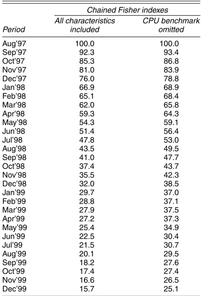
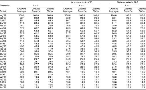
In Section 2 we present our basic model and derive an an-alytical expression for the bias due to the two sources noted earlier. Table 1 provides an empirical example of the bias ob-tained in the price index when an important characteristic is known to be omitted. For our data on desktop personal com-puter (PC) systems (more details of which are provided in Sec. 4.1), the table shows chained Fisher price indexes con-structed using a standard hedonic approach (left columns) and then again using the same approach but with the CPU bench-mark omitted (right columns). As shown in the table, the in-dexes with the CPU benchmark omitted exhibit substantial bias. Over just 29 months, the difference in overall inflation is ap-proximately 9%, with the biased indexes showing less deflation. This variation is larger than any variation that we were able to
Table 1. Left-Out Characteristics Bias
Chained Fisher indexes
achieve through alternative methods of constructing the index or alternative functional forms; thus we view it as potentially significant.
In Section 3 we show how factor analysis methods can be extended to construct a fairly general statistical test for the presence and even the dimension of the unobserved product characteristics. The intuition for this test is that for products with similar values of the unobserved characteristics, the price regression errors should move similarly over time. Next we show how to use similar methods to construct hedonic indexes that account for the unobserved characteristics. If the unob-served characteristic is one-dimensional, then it is possible to consistently estimate the hedonic surface (including recover-ing the unobserved characteristics) usrecover-ing a completely general functional form. If the unobserved characteristics are of two or more dimensions, then it is possible to consistently estimate the hedonic surface as long as there is a representation of the sur-face that is additively separable in the unobserved characteris-tics. Finally, we show that this methodology works in general if the unobserved characteristics are correlated with each other and, in certain cases, if they are correlated with the observed characteristics.
We apply our methods to a new dataset for desktop PCs. We find in these data that the dimension of the unobserved char-acteristics is likely to be either two or three. However, we also find that there were insufficient data to enable precise estimates of the price index when the unobserved characteristics were al-lowed to have dimension greater than one. Given the compre-hensiveness of the data, this result sheds doubt on the practical ability to correct price indexes in the multidimensional case. However, these difficulties were exacerbated in our data by
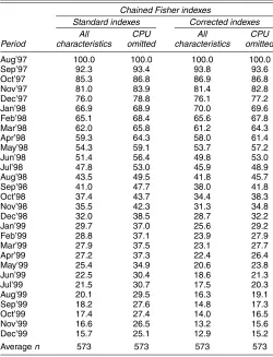
the extremely high rate of product turnover and the relatively high measurement error in the price data. Therefore, we believe that correcting for a multidimensional unobservable may be possible in other datasets with less-rapid product turnover and better price measurement. Based on the results of using a one-dimensional unobserved characteristic, we find that the stan-dard hedonic index is upwardly biased by approximately 1.4% per year, and that this bias is due primarily to selection. Specifi-cally, the unobserved characteristics for PCs are improving over time, and this upwardly biases the standard hedonic price index. We further test our estimation approach by leaving out an important characteristic (the CPU benchmark) and reestimating the price index. Although the standard hedonic index is severely biased in this case, our approach essentially removes the bias even if only a one-dimensional unobserved product character-istic is used (see Table 9 in Sec. 4.2.3). Thus, although the foregoing results suggest that correcting the index for a mul-tidimensional unobservable may be difficult, these results show that corrections based on a one-dimensional unobservable pro-vide a good approximation to the multidimensional case.
Our results suggest that there is a trade-off between the hedonic and matched-model approaches. Hedonic methods are better at capturing quality change and also can solve the prod-uct entry and exit problem of the matched-model approach. However, hedonic methods may be biased due to unobserved characteristics. Our approach of including unobserved product characteristics in the hedonic index can be viewed as achiev-ing a middle ground between the two standard approaches. Our approach also lies between the two standard approaches in terms of data requirements. A limitation of our approach is that products must be observed in several time periods, or several spatially separated markets, to estimate the vector of unobserved product characteristics. The number of periods re-quired depends on the dimension of the unobserved character-istics. This falls considerably short of that required to construct the matched-model index, for which every product must be ob-served in every period.
2. AN EXPRESSION FOR THE BIAS DUE TO UNOBSERVED CHARACTERISTICS IN
HEDONIC PRICE FUNCTIONS
2.1 Model and Notation
We assume that the econometrician has data fort=0, . . . ,T periods and, without loss of generality, we assume that the base period of the price index is periodt=0. It would not change anything in our analysis to consider instead eitherT spatially separated markets or a total ofT observations for a set of spa-tially separated markets over time. We assume that each com-modity,j, can be represented as a finite-dimensional vector of attributes. In most applications, the economist does not observe all of the product attributes relevant to the consumer. Therefore, in the model the economist perfectly observes the first K at-tributes, which we denote by the vectorxj=(xj1, . . . ,xjK), but
does not observe anL-vector of attributesξj=(ξj1, . . . , ξjL).
LetCt be the set of products in markett and denote the set of products that are available in both marketssandtbyCs,t= Cs∩Ct. LetFtbe the joint distribution of(x,ξ)in markettwith supportXt⊂RK+L, whereXtis assumed to be compact.
Implicit in the foregoing notation is the assumption that prod-ucts are readily identifiable in the sense that it is possible to identify the same product across different time periods t. Un-der this assumption, the entire vector of product characteristics,
(xj,ξ
j), is fixed across markets for each product. If a product’s
characteristics change between two periods, then we define the two products to be different products.
The assumption that a product’s characteristics stay fixed over time may be unrealistic in some industries. For example, if one characteristic of a product is the manufacturer’s reputation for providing good service, then that could change over time even if the physical aspects of the product do not. Examples of this might include the average hold time on a company’s cus-tomer service hotline.
2.2 Price Index Formulas
In this article we concentrate on what we believe are the most commonly used forms of the price index: plutocratic weighted average indexes with base period (Laspeyre) or reference pe-riod (Paasche) weights. We define the standard matched-model indexes as
Standard results show that ML
t is an upper bound and MPt is
a lower bound to the exact price index. These correspond to the classical bounds of Konus (1939) (see also Pakes 2003 for ways of deriving these bounds more generally). In Section 4 we find that, due to a high rate of product turnover, we must in-stead apply the “chained” versions of these indexes, in which the weights are constantly updated from one period to the next. Therefore, we also calculate chained Fisher indexes, because several authors (e.g., Aizcorbe, Corrado, and Doms 2003) have argued that the chained Fisher index provides a better approxi-mation to the true index in markets with high product turnover. Hedonic methods substitute prices predicted from the esti-mated hedonic surface, p(x), into (1) and (2) in the place of actual prices, not all of which are observed. The primary dif-ferences between hedonic methods arise in the details of how prices are predicted and whether the predicted prices should always be used or whether they should be used only where ac-tual prices are unavailable, or some combination of these op-tions. In this article we compare the matched-model indexes (MLt and MPt) with hedonic indexes (HLt and HPt) in which all of the prices are replaced with prices predicted by the hedonic index,
Our approach differs slightly from the methods proposed by Pakes (2003), which substitutes all prices in the numerator with prices predicted using the hedonic surface but uses actual prices in the denominator. It also differs from the method used by the Bureau of Labor Statistics (BLS), which uses a hybrid of the hedonic and matched-model methods that substitutes predicted prices only in cases where products drop out of the sample. However, our techniques can just as easily be applied to hedo-nic indexes of those forms. The alternative methods suggested by Pakes (2003) and used by the BLS are in part designed to al-low construction of the index under time constraints. We ignore these practical issues in this article.
2.3 An Analytical Expression of the Unobserved Characteristics Bias for the Linear Case
To better understand how unobserved characteristics lead to bias in the aggregate price index, in this section we derive an-alytical expressions for the bias in the index. Because this is difficult to do in general, we concentrate on the simple case in which the price function is linear. We thus write the price func-tion as
pjt=β0,t+x′jβx,t+ξ′jβξ,t, (5)
where bothxjandξjare vectors.
In characterizing the bias in HL, it is helpful to rewrite the
index as
where the functionspt(xj)are the hedonic surface in periodt,
which are only a function of the observed characteristics, as is common in practice.
Consider what happens if we estimate (5) using stan-dard techniques. Suppose, for the sake of simplicity, that we estimate (5) under the assumption thatξ andxare mean inde-pendent, Et[ξ|x] =Et[ξ] =µt. If the mean independence
as-sumption holds and there are a large number of observations in each period, then the parameter estimates obtained from theT regressions are
Note that the intercept captures the average change over time in both the price ofξand the mean ofξ.
We can now use (7) and (8), in conjunction with (6), to char-acterize the bias in H. The bias in the numerator of HLis
Bias
whereQ0is total sales of the good in the base period. Similarly,
the bias in the numerator of HPis
Bias
whereQtis total sales of the good in the reference period.
The expressions for the bias in the numerator involve two main terms. The first term depends on how much the mean ofξ
changes over time and thus reflects selection bias. If there is no selection, such that mean ofξ is constant over time, then the first term is 0. The second term reflects the extent to which the unobserved characteristics are revalued over time,(βξ,t−βξ,0).
If the value of the unobserved characteristics is constant over time then the second term is 0. These are the two sources of bias mentioned in Section 1. Note also that revaluation of the unob-served characteristics would not bias the index if there were no selection and the quantity-weighted mean ofξ were the same as its unweighted mean,µ. Interestingly, this suggests that if there were no selection problem, then using quantity weights in the hedonic regression would eliminate the unobserved character-istics bias in the index.
The expressions for the bias in the denominator involve sim-ilar terms. The bias in the denominator of HLis
Bias
whereas the bias in the denominator of HPis Bias
Den(HP)t=βξ,t
j∈Ct
(µt−ξj)′qjt. (12)
The bias in the denominator of the index reflects the extent to which the quantity-weighted mean of the unobserved charac-teristic differs from its unweighted mean. It is difficult to sign this bias in general, because the quantity weights depend on consumer tastes. Assuming that the unobserved characteristics carry positive prices, if demand is higher for goods with higher values of the unobserved characteristics, then the denominator is downwardly biased, leading to an upward bias in the index. Note also that the bias is constant over time for the Laspeyre index and is likely to be fairly constant for the Paasche index. This means that if the denominator is biased downward, then price changes in the index for all periods will be biased up-ward. Based on our experiences, our prior is that this source of bias is likely to be less important than the previous two.
The bias in the index as a whole is easiest to evaluate as-ymptotically because, by the Slutzky theorem, the bias in the index can then be evaluated by considering the biases in the nu-merator and denominator separately. This leaves three overall sources of bias, two in the numerator (selection and repricing of the unobserved characteristic) and one in the denominator (the difference between the quantity weighted mean ofξ and its unweighted mean). The bias in the index will reflect the sum of these three sources.
In our opinion, there are many industries in which the mean of the unobserved characteristics and the price of the unob-served characteristics are likely to change over time, particu-larly high-technology industries. In that case, it is likely that there would be unobserved characteristic bias in standard hedo-nic indexes.
3. MODELING UNOBSERVABLES IN THE HEDONIC PRICE FUNCTION
In this section we outline an approach to estimating hedo-nic price functions in the presence of unobserved characteris-tics. Our approach is similar to the factor analysis literature, especially the work of Lawley and Maxwell (1971), Goldberger (1974), and Cragg and Donald (1995, 1997), except that we have found it necessary to extend that work in several ways, most notably to account for selection.
3.1 The Hedonic Price Function
Bajari and Benkard (2003) provided a set of primitive con-ditions under which there exists a price surface, denoted by pt(xj,ξj), in each market t. For the remainder of the article
we implicitly rely on the results of their theorem in the sense that we assume that there exists a function mapping product characteristics to prices. Bajari and Benkard (2003) treatξjas
one-dimensional; however, extending the theorem to the case in whichξjisL-dimensional is straightforward. If the assump-tions of the theorem were to not hold, then the hedonic approach could still be viewed as an approximation to the truth. But we cannot say how good the approximation would be without mak-ing additional assumptions.
To simplify the analysis and estimation, we assume that the price function can be written as additively separable in the ob-served and unobob-served product characteristics and linear in the unobserved characteristics,
pjt=ft(xj)+β′ξ,tξj+νjt, (13)
whereft(·)is a function, possibly of unknown parametric form,
andνjt represents measurement error in the observed price.
Equation (13) places some restrictions on the functional form of the price function, but retains perhaps more generality than is first apparent. All of the analysis that follows is general to nonlinear transformations of the right-side and left-side vari-ables. In addition,ft(·)can be a general nonparametric function
within any one of those forms. Because we allow the unob-served product characteristics to be correlated with one another, higher-order terms inξ may appear as additional dimensions. Because our analysis is general to the case whereξ is corre-lated withx(if the relationship is stable over time; see Sec. 3.3), interactions betweenξ andxmay also appear as additional di-mensions. We allow for measurement error in prices, because in our experience with price data in I.O. applications, we have found that this can happen for various reasons, and furthermore, we believe it to be true in our data.
For ease of exposition, in this section we maintain several assumptions that we later relax. First, we assume that the un-observed product characteristics are mean independent of the observed product characteristics. This assumption is common in the hedonics literature implicitly and also in the literature on demand estimation explicitly. It seems likely that it is vio-lated to some extent in practice, so we show that it is possible to substantially relax this assumption in Section 3.3. Second, we assume that the measurement error is iid and independent ofxandξ. It is straightforward to generalize the specification of the measurement error in several ways, including AR(p), and heteroscedasticity of unknown form. We consider the latter case
here. Finally, the analysis is substantially easier to follow if we assume that there is no selection in the data; that is, we assume that the distribution ofξjis constant over time. We add selection
to the model in Section 3.2.
3.1.1 Estimating ft(·). Letǫjt≡β′ξ,tξj+νjt represent the
error terms in the period-by-period hedonic price regressions. Under the assumptions listed earlier,Et[ǫjt|x] =β′ξ,tµ, where
µ=E[ξj|xj]is a constant. Therefore, the functionsft(·)can be estimated using standard techniques. For example, if the para-metric form of the functionsft(·)were known, then they could
be estimated using least squares. Otherwise, kernel or series based nonparametric regression techniques could be used. Note that the ft(·)functions absorb the mean of the unobservable,
β′ξ,tµ, so at this point the functions can be estimated only up to an additive constant term. (If there is selection, then each func-tionft(·)absorbs the period mean of the unobservable,β′ξ,tµt.)
Because these estimation approaches are standard, we omit a detailed discussion of them and proceed as ifft(·)were known.
3.1.2 Estimatingβξ,t. What makes it possible to identify
and estimate the complete model (13) is the fact that this model places tight restrictions on the covariance matrix of the errors in the hedonic regressions,ǫjt. To derive those restrictions, we
first need to make some normalizations. The normalizations we use are standard to factor analysis and are without loss of gen-erality (see Lawley and Maxwell 1971 for a good discussion). We remind the readers that at this point we are maintaining the assumption that there is no selection. In the event that there is selection, we have to be careful in applying the normalizations; see Section 3.2 for details. We normalize the mean ofξ to be0, E[ξj] =0. We also normalizeξ to have covariance matrix IL
across all periods 0, . . . ,T. The reason that the normalizations are necessary is thatξ is not observable and thus has no inher-ent units. It is multiplied by a coefficiinher-ent vector that is also un-known. Thus neither the mean nor the variance ofξis identified separately from the coefficientsβξ. Importantly, knowledge of
the normalized coefficients is sufficient for construction of the price index.
Letǫjbe theT-vector of errors for productj. Then under the
assumptions given earlier,
≡E[ǫjǫ′j] =βξβ′ξ+σν2IT. (14)
Without any restrictions, E[ǫjǫ′j]has T(T+1)
2 unique elements.
However, our model contains onlyT∗L+1 parameters. Thus for small values of L, the model places significant restrictions on this matrix. In fact, it is possible to estimate the entire matrix of parametersβξ as long asL≤ T2 (approximately). Because
most price index applications have data for a large number of time periods or spatially separated markets, the model is typi-cally overidentified for reasonable values ofL.
Estimation ofβξ can be achieved in several ways. The
tra-ditional approach of the factor analysis literature (e.g., Lawley and Maxwell 1971) has been to assume normality for the un-observed product characteristics and then use maximum likeli-hood. However, such an approach would be inappropriate here, because the model provides us with only first- and second-moment information and nothing more. If we were to assume normality of the unobserved product characteristics, then, in conjunction with the normalization of their covariance matrix
to theILmatrix, we would be implicitly assuming full indepen-dence of the unobserved product characteristics. But we do not want to assume full independence, because we want to allow for functional form flexibility in (13). Thus we instead proceed using generalized method of moments (GMM), with the mo-ment conditions provided by (14). In a previous version of the article we used likelihood methods and found that they led to an overestimate of the number of unobserved product charac-teristics,L.
Assuming that there is no selection, the model can be esti-mated as follows. Let
Because (15) is the empirical counterpart to (14), our model gives us T(T2+1) unique moment conditions,
E[S] =. (16)
The natural GMM estimator would minimize a quadratic form in these moment conditions,
{ ˆβξ,σˆν} =arg min(vechS−vech)′A(vechS−vech), for some positive-definite weight matrix A. Under standard conditions, βˆξ and σˆν are consistent and asymptotically nor-mal for any positive-definite weight matrixA. For example, the Imatrix could be used. Also, under standard conditions,
√
J(vechS−vech)→N(0,V),
and it is well known that the optimal weight matrix to use in the GMM objective function isA=V−1(see Hansen 1982). In our application, the number of observations will typically vary by cell ofS, so the asymptotic approximations have to be corrected appropriately.
3.1.3 Hypothesis Tests for the Dimension L. The
forego-ing estimation algorithm is conditional on knowforego-ing the
dimen-sion L. Cragg and Donald (1997) showed that if the optimal
weight matrix is used, then the value of the objective function can also be used as a statistical test for the true dimension of the model. The difficulty in applying the approach of Cragg and Donald (1997) in our application comes in estimatingV. Typically, a consistent estimator ofVcan be obtained using the sample moments of ǫj. For example, an estimator for the
co-variance between the(q,r)and(s,t)elements ofSis given by
However, in our application, products tend to not last longer than about 12 months, so there are many combinations of
(q,r,s,t)for which there are very few or even no observations. Thus, although it is still possible to estimateV, it is not possi-ble to estimate it very well, in our experience not well enough to construct reliable hypothesis tests. One problem that we had was that the differing number of observations in every cell led to an estimate ofVthat was not positive definite due to sampling error and thus was not invertible to obtain the weight matrix. We solve this problem by using subsamples of data for which Vcan be estimated well.
A potential problem with these hypothesis tests is that the errors used to calculate the moment conditions in (16) are esti-mated and thus are not equal to the true error terms. Although this does not affect consistency of the index, the additional noise might influence the hypothesis tests toward causing false rejections (i.e., toward supporting too many unobserved fac-tors). The extent of the problem would likely depend on the number of first-stage observations and on the variance of the measurement error in price. One possible solution to this prob-lem would be to estimate the first and second stages jointly us-ing GMM. (We thank an anonymous referee for suggestus-ing this solution.) That is, the first stage consists of a set of OLS mo-ments (one set for each time period) given by
E[ǫjt|x] =0.
These moments could be combined with those in (16) into one large joint GMM estimation procedure. Hypothesis tests based on the joint GMM objective function would then account for first-stage estimation error. The problem with the joint approach is that it has a massive data requirement. Each time period in the first-stage estimation adds a set ofK moment conditions, leading to a total of NMOM=T∗(K+(T+1)/2)moments. To run hypothesis tests, it is necessary to obtain a good esti-mate of the variance covariance matrix of the moment condi-tions, which has NMOM∗(NMOM+1)/2 unique elements. For many datasets, including the one used in this article, this will not be possible. We discuss this issue further in Section 4.
3.1.4 Estimating ξ. The foregoing two-step approach
provides estimates of all of the model parameters. However, to construct price indexes, it is also necessary to estimate the vector of unobserved product characteristics for each product. The vector of errors for each productjcan be written as
ǫjt=β′ξ,tξj+νjt. (17)
At this point we assume that the parametersβ′ξ,t are known, because they have been estimated previously.
Becauseβξ,t is known and the measurement error is iid and
independent of everything, (17) becomes a standard linear re-gression model withβξ,t as the observed covariates andξj as
the unknown parameter vector. Estimation of this equation is straightforward via OLS. A problem likely to be encountered is that (17) can be estimated only for those products with prices observed inTj≥Lperiods and, depending on the variance of
the measurement error, can be estimated well only ifTjis large.
In that case, ifL>1, then in general it is not possible to esti-mateξj for all products, and it may be difficult to estimateξj
well unlessTjis large or the variance of the measurement error
is small. This also introduces some selection into the index, be-cause some products would have to be dropped in calculating the index.
In application,βξ,t is not known but is instead replaced by
a consistent estimator,βˆξ,t. This introduces finite-sample bias
into the estimates ofξ similar to that of measurement error in the standard regression model. Becauseβˆξ,tis consistent as the
number of products goes to infinity, this bias goes to 0 with the number of products. Provided that there is measurement error (σν2>0), consistency of ξˆj also requires that the number of
time periods (or spatially separated markets) become large for each product. Consistency ofξˆjthus would be obtained as both the number of products and the number of time periods become large.
3.2 Selection
An important problem with proceeding using the GMM ap-proach described earlier is that there is substantial selection in our data for PCs. As technology improves, lower-quality prod-ucts exit, and higher-quality prodprod-ucts enter. Thus, for example, it is unlikely that the products that we observe in period 1 are a random sample of products from the distribution of all products observed in all periods, as is required by the moment condi-tions in (16). In this section we allow there to be selection on both observed product characteristics,xj, and unobserved prod-uct characteristics,ξj. We continue to assume that the measure-ment error in price is iid and thus not subject to selection.
Selection introduces two main problems to the analysis. The first problem is that even if the mean of the unobserved prod-uct characteristics is normalized to 0 overall, the mean of the unobserved product characteristics is not necessarily 0 among products observed in any given period,µt≡Et[ξj|xj] =0. The
same is true among products observed in any pair of periods sandt. One way in which this shows up is that the errors from the hedonic price regressions,ǫj,t, will include a term in the
period mean of the unobserved characteristics,
ǫj,t=β′ξ,t(ξj−µt)+νjt.
This extra term must be accounted for when estimatingξj. This
can be done using multivariate and partitioned regression tech-niques or an equivalent iterative procedure.
The second problem caused by selection is that we observe the covariance of the errors in the price regression between two periods only for products observed in both periods. If selection influences these covariances, then it is impossible to calculate sample moments that correspond to the population moments given by (16). Formally, for any pair of periodss,t∈0, . . . ,T, the moments in (16) representE[ǫj,sǫj,t]. Instead, we observe
the sample counterpart to the population moment, E[ǫj,sǫj,t|
j∈Cs,t], where Cs,t represents the set of products observed in periodssandt. Therefore, if we were to proceed as described earlier and ignore the selection problem, then we may bias the estimates ofβξ as well as the statistical-dimension tests.
Our approach to handling selection is two-fold. First, when running the hypothesis tests for the dimensionL on subsam-ples as described earlier, instead of using all data points for all products observed at any point during the subsample, we reduce the data to a balanced panel. Formally, we choose a balanced panel,Cs,...,t, representing all products observed in all periods, s, . . . ,t. When running the statistical-dimension tests, we then use the moment conditions in (16), but only for products in the balanced panel,
E[S|j∈Cs,...,t] =.
Note that the fact that we are using a balanced panel means that we are using a selected group of products. For example, because these products were observed over the entire panel, they are likely to be better than products that dropped out at some point. The way in which this selection would show up is that the unobserved characteristics in the balanced panel would have a different (perhaps higher) mean and different covariance matrix than an unselected sample. However, the mean and
co-variance matrix are normalized away in the estimation, so the fact that they are different than what would be obtained with-out selection does not matter. What matters for the estimation is that the mean and covariance matrix are held constant across the moment conditions (the entire matrixS). Holding the selec-tion constant over the panel allows us to discern common move-ments in the price regression errors, which allows us to estimate the coefficients, βξ. As long as there are enough products in
the balanced panel to identify the coefficients, the selection no longer matters. The downside of the balanced-panel approach is that it forces us to throw out some of the information avail-able in the data; the upside is that it allows us to test for the dimensionLwhile allowing for selection without restrictions.
The balanced-panel approach does not allow us to estimate the price index as a whole, because very few (if any) products are observed in every period in the data. However, we can ex-tend the intuition of the balanced panel forward in several ways. Perhaps the easiest approach would be to chain together bal-anced panels for several subsamples of the data in order to con-struct the whole index. This approach should in principle work, but at the expense of not using all of the available information in the data. Instead, we propose using the moment conditions from overlapping balanced panels in conjunction with each other in order to estimate the overall index. However, in order to do this, we have to explicitly account for the varying selection across different panels.
Suppose that we apply the factor analysis normalizations rel-ative to the products in some group Cη, such that theξ’s for those products have mean0 and covariance matrixIL. For ex-ample, the groupCηcould be the balanced panel of all products observed in all periods 1, . . . ,10. Then, as above, these prod-ucts provide us with a series of moment conditions,
E[S|C1,...,10] =η≡βξβ′
ξ+σν2I.
Now, consider a second group of products,Cτ. For example, Cτ could be the balanced panel of all products observed in all periods 2, . . . ,11. If we allow the selection process to be com-pletely unrestricted, then we know nothing about the mean and variance ofξ among this second group relative to the normal-ization from the first group. However, we still have an equiva-lent set of moment conditions,
E[S|C2,...,11] =τ≡βξτβ′ξ+σν2I,
whereτ is the covariance matrix ofξjamong products inCτ. Because of the presence of the new parameters,τ, this second set of moment conditions does not provide as much information as the first. However, for small dimensionsL, they should still provide a great deal of information. For example, ifL=1 then these moment conditions are simply shifted by a constant rela-tive to the first group. In this manner we can use many moment conditions from successive overlapping balanced panels to es-timate the parametersβξ while allowing for selection without
restriction. Note that this procedure introduces new incidental parameters,τ, for each set of moment conditions used, and therefore increases the computational burden of the estimation.
3.3 The Nonindependent Case
We have already shown that if the unobserved product char-acteristics are correlated with each other but independent of the observed characteristics, then we can estimate the price in-dex by normalizing them to be uncorrelated with each other. In this section we consider the case where the unobserved prod-uct characteristics are also correlated with the observed prodprod-uct characteristics.
We consider the case where the functions ft(·) are
esti-mated using a nonparametric series estimator. This approach was suggested by Pakes (2003) and is also used in the empiri-cal section (Sec. 4) of this article. It also nests many parametric approaches, including linear, semilog, and log–log, and can be viewed as an approximation to other nonparametric approaches. In that case, the price equation can be written as
pjt=β0,t+β′x,tφ(xj)+β′ξ,tξj+νjt, (18)
whereφ(xj)is aM×1 vector of basis functions ofxjandβx,t
is aM×1 vector of parameters.
Without loss of generality,ξjcan be written as,
ξj=µt+γtφ(xj)+ζjt, (19)
whereEt[ζjt|φ(xj)] =0 andγt is aL×M matrix of
parame-ters. The expression (19) represents the periodtprojection ofξj
on φ(xj)with respect to the periodt sampling distribution of
(xj,ξ
j). [For clarification,µtandγtare the coefficients from a
regression ofξjonφ(xj)for all products observed in periodt.] In general, the relationship betweenξjandφ(xj)may vary over time, depending on such factors as changes in production tech-nology and selection. But suppose that the projection were sta-ble over time, such that
ξj=γ φ(xj)+ζj, (20) whereEt[ζj|φ(xj)] =µtfor all time periods,t. Then combining
(18) and (20) gives
pjt=β0,t+(β′x,t+β′ξ,tγ )φ(xj)+βξ′,tζj+νjt. (21)
This model is analogous to that estimated earlier for the inde-pendent case. Thus, using the approach outlined earlier, we can consistently estimate the quantities β0,t,(β′x,t+β′ξ,tγ ),βξ,t,
and ζj, under the correct assumption that Et[ζj|φ(xj)] =µt.
The quantities βx,t, γ, and ξj are not separately identified/
estimable using this approach. However, we do not need these quantities to evaluate pt(xj,ξj). The estimable quantities are
sufficient for evaluating this function and thus are sufficient for construction of the hedonic price index. Thus, as long as the re-lationship betweenξjandxjis stable over time, the estimation approach described in the previous section provides consistent estimates of the price index.
Although it is substantially more general than assuming that they are independent, the assumption that the relationship be-tweenξjandxjis stable over time is somewhat restrictive,
par-ticularly if we were considering long panels. However, it would also be possible to use balanced panels in the first-stage hedo-nic regressions to solve the correlation problem more generally. The reason that balanced panels would work is the same as be-fore. They hold the set of products fixed over time, thus making the relationship betweenξjandxjfixed over time.
4. EMPIRICAL RESULTS
4.1 Data
Our data come from thePC Data Retail Hardware Monthly Report and include quantity sold, average sales price, and a long list of machine characteristics for desktop computers sold over a 29-month period from August 1997 to December 1999. This dataset reportedly covers approximately 75% of U.S. retail computer sales. The price data are collected from cash register receipts, and the dataset is constructed by taking total sales of each product over a month and dividing by quantity sold. The dataset thus represents the average retail sales price of the ma-chine in that month. In working with the raw data, we discov-ered two problems that we felt we needed to address. First, the data for machines with very few sales was highly variable from month to month. Second, sometimes machines are recorded as having been sold at very low prices (e.g., $.01) when they were in fact taken off the books for other reasons, such as because the unit was stolen. Thus, to remove both of these problems, we dropped all price observations for units that sold fewer than 10 units in a given period. After dropping these observations, 3,853 machines remained from an original sample of approxi-mately 8,000.
The characteristics data included 65 product characteristics, including 23 processor-type dummies and 9 operating system-type dummies. To reduce the dimension of the characteristics space, rather than use the 23 processor-type dummies and the speed rating of the chip as separate characteristics, we instead obtained CPU benchmarks for each machine fromThe CPU
Scorecard(www.cpuscorecard.com). Despite having
consider-able variation, a regression of the CPU benchmark variconsider-able on processor dummies interacted with chip speed had an R2 of .995, justifying its use.
Of the remaining 41 characteristic fields, we eliminated those fields that either were not reliable (not always recorded) or ap-plied only to a handful of machines. Despite the need to drop several of the characteristics fields, we were left with an ex-tremely rich set of characteristics. The final characteristics set included nine operating system dummies (Win 3.11, Win 3.1, NT 3.51, NT3.2, NT 4.0, NT, Win 98, Win 95, other) plus CPU benchmark, MMX, RAM capacity, hard drive capacity, SCSI, CDROM, DVD, modem, modem speed, NIC, monitor dummy, monitor size, zip drive, desktop (versus tower), refurbished, dual hard drive, and dual processor, for a total of 26 charac-teristics.
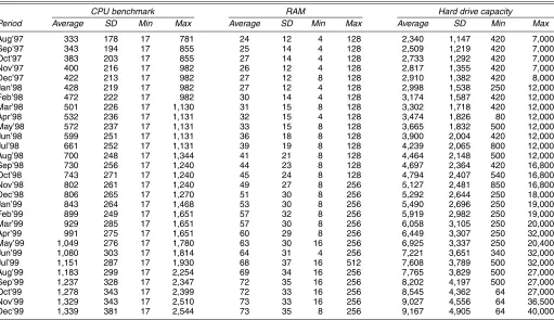
Tables 2 and 3 contain summary statistics for the final dataset. Table 2 shows that there are approximately 600 ma-chines per month in the data, representing an average of approx-imately 300,000 units sold. The sales-weighted average price of machines drops by approximately 40% over the 29-month period. The unweighted average price is generally higher, but moves similarly. At the same time, Table 3 shows that sales-weighted average CPU benchmark and sales-sales-weighted average hard drive capacity both rise by approximately a factor of four, whereas sales-weighted average RAM rises by approximately a factor of three. To summarize, prices for a constant-quality ma-chine are dropping rapidly, but consumers are also rapidly
Table 2. Summary of PC Data
Unique Total Average price Average price Period machines sales (unweighted) (sales-weighted)
Aug’97 577 226,029 1,396 1,422 Sep’97 556 239,417 1,408 1,437 Oct’97 562 211,610 1,411 1,423 Nov’97 517 265,070 1,358 1,351 Dec’97 524 345,153 1,308 1,321 Jan’98 572 328,028 1,224 1,200 Feb’98 525 331,262 1,172 1,217 Mar’98 614 371,337 1,187 1,194 Apr’98 601 260,173 1,206 1,179 May’98 547 210,834 1,182 1,134 Jun’98 660 278,002 1,160 1,111 Jul’98 563 250,110 1,156 1,133 Aug’98 615 345,183 1,177 1,092 Sep’98 649 393,909 1,131 1,113 Oct’98 647 296,737 1,128 1,032 Nov’98 563 428,776 1,046 1,099 Dec’98 644 592,138 1,042 995 Jan’99 593 406,644 981 1,028 Feb’99 569 371,586 998 1,056 Mar’99 675 452,156 1,025 1,046 Apr’99 635 313,716 977 1,061 May’99 608 285,353 968 1,033 Jun’99 692 378,476 947 1,002 Jul’99 614 330,798 878 1,020 Aug’99 616 478,200 841 992 Sep’99 672 571,820 848 953 Oct’99 710 379,487 866 914 Nov’99 661 484,269 861 925 Dec’99 747 664,983 912 879
stituting toward higher-quality machines. The net result is that average purchase prices still drop by 50% over the 29-month period.
Table 3 shows that, despite the fact that our data cover only 29 months, there is considerable shift in the boundaries of the characteristics space over time. The shift in the minimum set of characteristics available is only slight. However, there is a considerable shift upward in the maximum characteristics avail-able, particularly with respect to CPU benchmark and hard drive capacity. Table 3 also leaves out some shifts in the charac-teristics space with respect to the other product characcharac-teristics; for example, in our data, Windows NT 3.51 is unavailable after May 1998.
4.2 Price Index Calculations
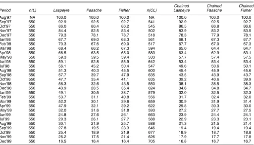
4.2.1 Standard Indexes. Table 4 lists matched-model
price indexes calculated using the final dataset. Even though our data is quite high-frequency relative to that used by the BLS, the standard matched-model indexes are quite unreliable here, because there is so much attrition in the sample. The standard indexes suffer from a selection bias, present even in the initial periods, as well as from considerable noise in later periods due to there being so few matched products (note the drop from No-vember 1999 to December 1999). In our opinion, Table 4 shows how difficult it is to construct a matched-model price index for a fast-paced high-technology industry like PCs. Even in such a short span as 2 years and even using a very comprehensive dataset covering nearly 4,000 machines, it is nearly impossible to use the matched-model method to construct a reliable price index. On the other hand, there are sufficient observations com-mon to any two neighboring periods so that the chained indexes do not suffer from the same sampling noise problem. However,
Table 3. Summary of Product Characteristics
CPU benchmark RAM Hard drive capacity
Period Average SD Min Max Average SD Min Max Average SD Min Max
Aug’97 333 178 17 781 24 12 4 128 2,340 1,147 420 7,000 Sep’97 343 194 17 855 25 14 4 128 2,509 1,219 420 7,000 Oct’97 383 203 17 855 27 14 4 128 2,733 1,292 420 7,000 Nov’97 400 216 17 982 26 12 4 128 2,817 1,355 420 7,000 Dec’97 422 213 17 982 27 12 8 128 2,910 1,382 420 8,000 Jan’98 428 219 17 982 27 12 4 128 2,998 1,538 250 12,000 Feb’98 472 222 17 982 30 14 4 128 3,174 1,587 420 12,000 Mar’98 501 226 17 1,130 31 15 8 128 3,302 1,718 420 12,000 Apr’98 532 236 17 1,131 32 15 4 128 3,474 1,826 80 12,000 May’98 572 237 17 1,131 33 15 8 128 3,665 1,832 500 12,000 Jun’98 599 251 17 1,131 36 18 8 128 3,900 2,004 420 12,000 Jul’98 661 252 17 1,131 39 19 8 128 4,239 2,065 800 12,000 Aug’98 700 248 17 1,344 41 21 8 128 4,464 2,148 500 12,000 Sep’98 730 256 17 1,240 44 23 8 128 4,697 2,364 420 16,800 Oct’98 743 271 17 1,240 45 24 8 128 4,794 2,407 540 16,800 Nov’98 802 261 17 1,240 49 27 8 256 5,127 2,481 850 16,800 Dec’98 806 265 17 1,270 51 30 8 256 5,292 2,644 250 18,000 Jan’99 843 264 17 1,468 53 30 8 256 5,490 2,696 250 19,000 Feb’99 899 249 17 1,651 57 32 8 256 5,919 2,982 250 19,000 Mar’99 929 285 17 1,651 57 30 8 256 6,058 3,105 250 20,000 Apr’99 991 275 17 1,651 60 29 8 256 6,449 3,307 250 32,000 May’99 1,049 276 17 1,780 63 30 16 256 6,925 3,337 250 20,400 Jun’99 1,080 303 17 1,814 64 31 4 256 7,221 3,651 340 32,000 Jul’99 1,151 287 17 1,930 68 37 16 512 7,608 3,789 500 32,000 Aug’99 1,183 299 17 2,254 69 34 16 256 7,765 3,829 500 27,000 Sep’99 1,237 328 17 2,347 72 35 16 256 8,202 4,197 500 27,000 Oct’99 1,278 343 17 2,399 72 33 16 256 8,545 4,362 64 27,000 Nov’99 1,329 343 17 2,510 73 33 16 256 9,027 4,556 64 36,500 Dec’99 1,339 381 17 2,544 73 35 8 256 9,167 4,905 64 40,000
NOTE: Averages and standard deviations (SDs) are sales-weighted.
Table 4. Matched-Model Indexes
Chained Chained Chained
Period n(L) Laspeyre Paasche Fisher n Laspeyre Paasche Fisher
Aug’97 NA 100.0 100.0 100.0 NA 100.0 100.0 100.0 Sep’97 425 96.0 96.2 96.1 425 96.0 96.2 96.1 Oct’97 353 91.2 91.7 91.5 405 91.9 92.6 92.3 Nov’97 294 82.5 81.1 81.8 412 85.5 84.1 84.8 Dec’97 266 77.6 76.6 77.1 400 81.3 79.5 80.4 Jan’98 253 70.3 72.0 71.2 405 75.8 73.8 74.8 Feb’98 206 67.3 67.8 67.5 416 69.7 69.7 69.7 Mar’98 198 60.0 59.8 59.9 431 67.0 66.0 66.5 Apr’98 172 59.0 63.2 61.0 473 62.6 61.9 62.2 May’98 122 56.8 62.5 59.6 427 58.8 58.6 58.7 Jun’98 147 50.7 56.0 53.2 439 53.8 52.6 53.2 Jul’98 88 49.7 53.6 51.6 429 49.3 48.8 49.1 Aug’98 83 50.6 46.8 48.7 443 46.1 46.0 46.1 Sep’98 91 65.1 43.7 53.3 453 43.7 43.3 43.5 Oct’98 103 44.9 44.9 44.9 478 39.7 40.4 40.1 Nov’98 49 57.3 68.9 62.8 429 37.1 37.6 37.4 Dec’98 73 36.4 41.3 38.8 459 35.5 35.8 35.7 Jan’99 45 53.3 45.0 49.0 447 31.8 33.3 32.5 Feb’99 27 77.9 59.7 68.2 419 30.4 32.3 31.3 Mar’99 37 87.9 98.2 92.9 449 29.0 30.6 29.8 Apr’99 12 86.9 105 95.7 471 27.7 29.1 28.4 May’99 4 16.3 33.5 23.4 426 26.6 28.0 27.3 Jun’99 13 14.4 47.7 26.2 459 24.9 26.2 25.6 Jul’99 1 65.5 65.5 65.5 468 23.0 24.6 23.8 Aug’99 2 23.9 47.9 33.8 459 21.8 22.9 22.4 Sep’99 1 65.4 65.4 65.4 473 20.8 21.6 21.2 Oct’99 2 62.3 61.2 61.7 499 19.2 20.6 19.9 Nov’99 2 58.3 58.9 58.6 509 18.1 19.8 18.9 Dec’99 5 13.1 20.1 16.3 532 17.7 19.5 18.5
NOTE: n(L) is the number of units used to construct the Laspeyre index.nis the number of units used to construct the chained indexes.
with the chained indexes there is still a potential selection prob-lem with respect to which products remain in the market from period to period.
Table 5 shows standard hedonic indexes calculated using the same dataset. In implementing the hedonic indexes, we needed to choose a baseline functional form. In the spirit of
nonpara-Table 5. Standard Hedonic Indexes
Chained Chained Chained Period n(L) Laspeyre Paasche Fisher n(CL) Laspeyre Paasche Fisher
Aug’97 NA 100.0 100.0 100.0 NA 100.0 100.0 100.0 Sep’97 550 92.9 92.5 92.7 541 92.9 92.5 92.7 Oct’97 550 86.0 86.4 86.2 545 86.5 86.8 86.6 Nov’97 550 84.4 82.5 83.4 502 83.9 83.2 83.5 Dec’97 550 79.3 78.1 78.7 518 78.3 77.9 78.1 Jan’98 550 67.7 69.0 68.3 561 68.1 67.3 67.7 Feb’98 550 70.3 67.6 69.0 517 67.7 67.0 67.3 Mar’98 550 68.4 66.2 67.3 594 65.0 64.4 64.7 Apr’98 550 66.5 63.5 65.0 583 63.4 62.9 63.1 May’98 550 59.3 59.5 59.4 533 57.7 57.4 57.5 Jun’98 550 59.1 52.8 55.9 642 53.4 53.4 53.4 Jul’98 550 56.1 45.2 50.4 547 49.6 50.6 50.1 Aug’98 550 51.3 40.3 45.5 600 45.4 45.9 45.6 Sep’98 550 57.7 39.7 47.9 635 43.5 43.9 43.7 Oct’98 550 47.7 35.4 41.1 635 39.2 40.6 39.9 Nov’98 550 58.3 32.6 43.5 550 38.1 38.5 38.3 Dec’98 550 43.9 28.5 35.4 624 34.6 34.8 34.7 Jan’99 550 49.1 30.5 38.7 579 32.0 32.5 32.3 Feb’99 550 53.7 31.1 40.8 556 31.7 32.4 32.0 Mar’99 550 52.2 30.1 39.6 659 30.9 31.9 31.4 Apr’99 550 47.9 32.1 39.2 622 29.8 30.3 30.0 May’99 550 32.0 31.6 31.8 593 27.2 27.7 27.5 Jun’99 550 24.8 27.6 26.1 663 23.9 24.4 24.1 Jul’99 550 29.3 26.1 27.7 588 22.9 23.3 23.1 Aug’99 550 30.1 21.9 25.7 588 21.3 21.5 21.4 Sep’99 550 27.8 19.5 23.3 646 19.4 19.4 19.4 Oct’99 550 25.4 18.9 21.9 677 18.9 18.7 18.8 Nov’99 550 26.2 17.5 21.4 626 17.9 17.7 17.8 Dec’99 550 16.5 16.4 16.4 705 16.8 16.7 16.7
NOTE: The functional form is semilog.R2ranges from .40 to .78.n(L) is number of units used to construct the Laspeyre index.n(CL) is number of units used for the chained Laspeyre index.
metric estimation, when choosing the baseline functional form, our goal was to find the functional form that provided the best fit for the hedonic surface. We tried several functional forms, including linear, semilog [in which only the left side (price) is in log form] and log–log. An analysis of the residuals from these functional forms over several time periods revealed that log-log provided a very poor fit. The linear form fit the high-end machines well, but did not fit the low-high-end machines well (vastly underpredicting price). The semilog fit the low-end ma-chines well, but showed some slight problems at the high end (slightly underpredicting price). We judged that the best of the three forms was the semilog, and so we proceeded using this as our baseline form. Our judgement was based on a series of statistical tests as well as “eyeing” the fit via residual charts. These results are also consistent with the arguments of Diew-ert (2003), which argues that the left-side variable in hedonic regressions should be in log form.
Coefficients in the hedonic regressions generally had the ex-pected signs, the main exception being the modem variable, which consistently was estimated to have a negative coefficient. We speculate that this may be due to the fact that computers with modems are generally intended for home use and may be of lower average quality in other respects that are not ob-served. Individual coefficients are not reported, because there were 29 regressions with approximately 26 coefficients each, for a total of 754 coefficient estimates.
The standard hedonic index and the matched-model index are quite different over some ranges (e.g., from August 1997 to September 1997), probably reflecting the selection problem in the matched-model indexes. However, their movement over the whole sample is surprisingly similar. This result is contrary to the results of Pakes (2003), who found that the selection prob-lem is so bad that the matched-model indexes actually rise for some periods instead of falling. We do not know for sure why our results differ so much in this respect; however, we speculate that selection is not nearly as bad a problem in monthly data as it is in yearly data. In our data, it is typical for more than 90% of the products in one month to be observed in the next month, whereas typically fewer than 10% are observed 12 months later. (However, the fact that 90% of the products are observed from one month to the next does not preclude selection being a bad problem.) From a policy standpoint, this evidence may suggest that it is worthwhile to use higher-frequency data in industries that have a lot of product turnover. Note that our results also show slightly faster rates of decline than those of Aizcorbe et al. (2003) for the period in which the data overlap.
We found that the standard (i.e., nonchained) hedonic in-dexes were subject to some variability with respect to changing the functional form of the hedonic price function. This variabil-ity arises because of the fact that the product space is changing over time. Because PCs are improving over time, when calcu-lating the price index for periods that are far apart in time, it is typically necessary to extrapolate the hedonic price function outside the range of characteristics space on which it was es-timated. We found that this introduced substantial variability into the index to the point where we are not confident in the results of the nonchained indexes for even the best of the func-tional forms. On the other hand, changing the funcfunc-tional form had very little effect on the chained indexes, because very little extrapolation was needed between adjacent periods.
Despite the fact that our dataset contains many characteris-tics, we found that theR2statistics in the hedonic regressions ranged from .40 to .78. Although these were lower than ex-pected, they are in the same range as those given by Pakes (2003), and they are lower than those of Holdway (2001). How-ever, Holdway (2001) used data obtained solely from large web-based retailers and hence likely to be holding many unobserved factors constant. This result suggests that either there are still some important characteristics, such as sales outlet or quality, that we do not observe or there is substantial measurement error in prices.
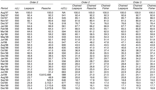
Table 6 gives standard hedonic indexes similar to those de-scribed earlier, except that a polynomial series was used on the right side (as suggested in Pakes 2003), but retaining the semi-log form. In general these indexes resulted in better in sample fit of the hedonic function, particularly for those periods in which fit was previously the poorest. Many of the coefficients on the second-order terms were also statistically significant. However, this improvement came at some cost with respect to prediction near the boundaries of the sample in characteristics space. The result is that even with just a second-order polynomial, there are some wild fluctuations in the standard price indexes (see the Paasche price index for July–December 1999). We found that going to higher-order polynomials further improves the fit of the model, but makes the price index even wilder. Again, the problem was not as bad for the chained indexes, as can be seen in the table.
Because of the unreliability of the nonchained indexes here and earlier, in the next section we report results only for the chained indexes. For similar reasons (sampling error), we use the second-order polynomial indexes, rather than the third-order ones, as our base case index.
4.2.2 The Multidimensional Case. Table 7 reports
p-values for hypothesis tests based on the GMM objective func-tion for various values of L. The first three columns report the baseline tests run for iid measurement error and three sub-samples of approximately 10 periods that divide the data into roughly three pieces. We chose to use 10 period subsamples because 10 periods provided sufficient degrees of freedom to run tests for values ofLup to about five while maintaining suf-ficient observations in the balanced panel. Tests with smaller and larger subsamples generated similar results, as did tests us-ing different subsamples of 10 periods. Results from the three tests are slightly inconsistent, with the early periods requiring a higher dimensional unobservable, but generally imply that the true dimensionLis greater than or equal to four.
Because the coverage of the data changes slightly over the panel, and because the variance in PC prices generally falls over our sample, we were concerned that the measurement error variance might not be constant over time. Thus, we reran the hy-pothesis tests, allowing for heteroscedasticity of unknown form in the measurement error. Relative to the baseline tests, to al-low for heteroscedasticity of unknown form, we need only run the same estimation procedure, but throwing out the moment conditions corresponding to the diagonal of the covariance ma-trix in (16). Allowing for heteroscedasticity of unknown form, all three tests suggest that we cannot reject that the true value is L=3. If we allow L to be large, then it is impossible to test whether the measurement error is heteroscedastic or not,
Table 6. Nonparametric Hedonic Indexes
Order 2 Order 2 Order 3
Chained Chained Chained Chained Chained Chained Period n(L) Laspeyre Paasche n(CL) Laspeyre Paasche Fisher Laspeyre Paasche Fisher
Aug’97 NA 100.0 100.0 NA 100.0 100.0 100.0 100.0 100.0 100.0 Sep’97 550 92.4 92.2 541 92.4 92.2 92.3 92.6 92.7 92.6 Oct’97 550 84.5 85.4 545 85.1 85.5 85.3 85.7 86.4 86.0 Nov’97 550 82.1 80.6 502 81.6 80.4 81.0 81.5 80.9 81.2 Dec’97 550 77.6 75.8 518 76.7 75.4 76.0 76.6 76.2 76.4 Jan’98 550 64.6 66.9 561 67.7 66.2 66.9 67.7 68.2 67.9 Feb’98 550 66.8 64.3 517 66.0 64.3 65.1 65.5 65.8 65.6 Mar’98 550 64.6 62.3 594 62.9 61.2 62.0 62.0 62.7 62.4 Apr’98 550 63.5 59.2 583 60.1 58.5 59.3 59.5 60.0 59.8 May’98 550 56.4 54.6 533 54.9 53.6 54.3 54.4 54.9 54.7 Jun’98 550 56.0 50.1 642 51.6 51.3 51.4 51.2 52.3 51.8 Jul’98 550 54.7 45.5 547 47.4 48.2 47.8 47.1 49.6 48.3 Aug’98 550 50.3 40.0 600 43.5 43.5 43.5 43.2 44.5 43.8 Sep’98 550 59.2 38.8 635 40.9 41.0 41.0 40.6 41.9 41.3 Oct’98 550 47.4 41.5 635 36.9 38.0 37.4 36.5 38.3 37.4 Nov’98 550 60.5 38.9 550 35.4 35.6 35.5 35.3 39.7 37.4 Dec’98 550 46.8 38.5 624 31.9 32.0 32.0 32.7 36.9 34.7 Jan’99 550 53.9 35.7 579 29.7 29.7 29.7 30.6 34.2 32.4 Feb’99 550 63.2 36.1 556 28.9 28.7 28.8 29.7 33.1 31.4 Mar’99 550 59.4 35.9 659 28.0 27.7 27.9 28.8 32.1 30.4 Apr’99 550 54.2 36.0 622 27.6 26.8 27.2 28.4 31.2 29.8 May’99 550 31.2 32.0 593 25.8 25.0 25.4 26.2 28.9 27.5 Jun’99 550 20.6 31.2 663 22.8 22.1 22.5 22.9 25.2 24.0 Jul’99 550 23.8 13,612,488 588 21.9 21.0 21.5 22.1 24.1 23.1 Aug’99 550 23.7 48.9 588 20.6 19.6 20.1 20.8 22.4 21.6 Sep’99 550 22.1 523.9 646 18.7 17.8 18.2 18.8 20.3 19.6 Oct’99 550 24.8 2,153.1 677 18.0 16.9 17.4 18.0 19.4 18.7 Nov’99 550 25.0 2,115.6 626 17.2 16.1 16.6 17.1 18.3 17.7 Dec’99 550 13.4 5,073.8 705 16.2 15.3 15.7 16.2 17.6 16.8
NOTE: The functional form is semilog with polynomial series.R2ranges from .50 to .79.n(L) is the number of units used to construct the Laspeyre index.n(CL) is the number of units used for
the chained Laspeyre index. The order is polynomial order.
because the model can always match the data equally well by increasingL. However, in our opinion, given the comprehen-siveness of the characteristics data, the result thatL=3 is more reasonable than those discussed earlier. We also find further support for heteroscedastic measurement error later.
We also worried that the large-sample tests may overreject due to the fact that first-stage estimates are used in place of the true error terms in the hypothesis tests. Because our data did not contain sufficient data points to allow joint estimation of the two stages, we instead simulated finite-sample critical values using the coefficient estimates obtained later and the assumption that
Table 7. p-Values for Dimensionality Tests
Homoscedastic ME Heteroscedastic ME Subsample (months): 1–10 11–20 21–29 1–10 11–20 21–29
Large-sample test: Dimension (L)
0 0 0 0 0 0 0
1 0 0 0 0 0 0
2 0 0 0 0 0 .046
3 0 .001 .006 .147 .913 .958 4 .001 .244 .749 .757 .963 5 .025 .248
Small-sample tests: Dimension (L)
0 0 0 0 0 0 0
1 0 0 0 0 .003 0 Number of 93 58 137 93 58 137 observations
NOTE: The blank areas indicate too few degrees of freedom to calculate.
both the unobserved characteristics and the measurement er-ror were normally distributed. The results of these tests showed that the finite-sample critical values were indeed larger than the asymptotic critical values. However, as shown in Table 7, the hypothesis thatL=1 is still rejected in all cases. We therefore conclude that in this dataset,L∈ {2,3}.
Table 8 gives chained price indexes constructed for theL=0 andL=1 cases. We estimated theL=1 case using the mo-ments from all balanced panels of length 3, 4, 5, 9, and 10 periods. We found that the results were extremely stable over choices of which panel lengths to use (to within .1 in the over-all index). The primary reason for choosing these period lengths was a trade-off between efficiency and computational burden. The more period lengths that we use, the more efficient the estimates, but at the expense of higher computational burden. We wanted to include several short panels because they gener-ally have more data points, as well as several long panels so as to incorporate information from periods that are far apart in the data. Comparing theL=0 andL=1 cases, we find that correcting for unobserved characteristics substantially reduces the index, by 2.9% over the 29-month period for the Fisher in-dex. The reason for this bias is primarily selection. We find that the unobserved characteristics are substantially improving over time (i.e., their normalized mean moves steadily upward from approximately−.3 to .2 over the period). The standard hedonic index (L=0) absorbs the mean unobserved characteristic in each period into the intercept of the price function. Then when predicting the prices of goods from previous periods that were not observed in later ones, it overpredicts their prices, raising