Full Terms & Conditions of access and use can be found at
http://www.tandfonline.com/action/journalInformation?journalCode=ubes20
Download by: [Universitas Maritim Raja Ali Haji] Date: 12 January 2016, At: 23:28
Journal of Business & Economic Statistics
ISSN: 0735-0015 (Print) 1537-2707 (Online) Journal homepage: http://www.tandfonline.com/loi/ubes20
Testing and Valuing Dynamic Correlations for
Asset Allocation
Robert Engle & Riccardo Colacito
To cite this article: Robert Engle & Riccardo Colacito (2006) Testing and Valuing Dynamic Correlations for Asset Allocation, Journal of Business & Economic Statistics, 24:2, 238-253, DOI: 10.1198/073500106000000017
To link to this article: http://dx.doi.org/10.1198/073500106000000017
Published online: 01 Jan 2012.
Submit your article to this journal
Article views: 251
View related articles
Testing and Valuing Dynamic Correlations
for Asset Allocation
Robert ENGLE
New York University, Stern School of Business, New York, NY 10003 (rengle@stern.nyu.edu)
Riccardo COLACITO
New York University, Department of Economics, New York, NY 10003 (rc652@nyu.edu)
We evaluate alternative models of variances and correlations with an economic loss function. We construct portfolios to minimize predicted variance subject to a required return. It is shown that the realized volatility is smallest for the correctly specified covariance matrix for any vector of expected returns. A test of relative performance of two covariance matrices is based on work of Diebold and Mariano. The method is applied to stocks and bonds and then to highly correlated assets. On average, dynamically correct correlations are worth around 60 basis points in annualized terms, but on some days they may be worth hundreds.
KEY WORDS: Dynamic conditional correlation; Forecast evaluation; Generalized autoregressive con-ditional heteroscedasticity.
1. INTRODUCTION
The literature on time series models for covariance matrices is now extremely large, with many proposed specifications and many empirical examples. However, explicit comparisons be-tween methods have been hampered by the multitude of metrics to use in forming the comparisons. The distance between two covariance matrices is not well defined, and it is certainly not obvious that all elements of this difference should be treated as equally important. The performance of any fixed-weight port-folio can be compared as a univariate problem; however, this leaves open the question of which portfolios to use.
In this article an asset allocation perspective is introduced to measure the value of covariance information. The realized volatility of optimized portfolios is considered, where the port-folios are chosen to minimize predicted variance subject to a required return and the analysis is carried out for a full range of hypothetical required returns. In each case there is a test for correct specification of the covariance forecast. It is shown that the realized volatility is smallest for the correctly specified co-variance matrix for any vector of expected returns. This leads to tests of the relative performance of two covariance matrices based on work of Diebold and Mariano (1995). The value of correct information is viewed as the increase in required return that can be achieved with no increase in volatility.
This framework is a natural extension of univariate forecast evaluation. Many univariate volatility comparisons consider simply the mean squared error between future realized volatil-ity and model forecasts. This comparison does not have an eco-nomic basis. Overestimates and underestimates of volatility of the same magnitude are treated as equally serious, even though the underestimate could be so low that volatility was predicted to be zero. Because realized volatility is a skewed distribution, the mean is only one measure of the center. In many cases the variances are compared and are even more sensitive to high-volatility shocks. Recently, Andersen and Bollerslev (1997) im-proved this metric by obtaining better estimates of realized volatility based on intradaily data. This does not improve the economic underpinning of the criterion, however.
In the univariate case, there have been several approaches to developing economic loss functions. West and Cho (1995) let
a mean variance utility maximizer choose between the riskless and risky asset and argued that the best model is the one that achieves the highest utility for its investor. Engle, Kane, and Noh (1996) let investors price options with different volatility models and see which strategy ends up with positive profits. If one investor thinks that the volatility will be higher than an-other, then he or she will be long astraddle, while the other will take the short position. Over a long period, the best volatility forecast should take money from inferior ones.
In the classical asset allocation framework, an investor is as-sumed to choose portfolio weights, including a riskless asset, to minimize variance subject to a required return constraint. Investors with different covariance forecasts and different ex-pected return forecasts will hold different portfolios. A low re-alized utility could be the result of the failure of either of these assumptions; it is essential to distinguish between these cases. Because it is impossible to know the true vector of expected returns, how can covariance matrices be compared?
A large body of literature has investigated the effectiveness of different static covariance matrices in asset allocation. Ini-tially, Elton and Gruber (1973) examined this problem and were the first to use ex-post means in the comparison. Subsequently, many authors have followed this route (see Cumby, Figlewski, and Hasbrouck 1994; Fleming, Kirby, and Ostdiek 2001, 2003). This method does not avoid the problem, however, because ex-pected returns are not the same as realized mean returns. In fact, they may be quite different, as, for example, when returns are on average negative. It furthermore biases the optimal portfo-lios to assets with high ex-post returns even though an optimal portfolio might not hold many of these assets. Other approaches restricted attention to minimum variance portfolios or portfo-lios that are minimum variance around a benchmark (e.g., Chan, Karceski, and Lakonishok 1998). This formulation is equivalent to assuming that all assets have the same expected returns—an unattractive assumption for stock and bond allocations or any
© 2006 American Statistical Association Journal of Business & Economic Statistics April 2006, Vol. 24, No. 2 DOI 10.1198/073500106000000017
238
other case where the risk and return characteristics are quite different across the assets.
The goal of this article is to isolate the effect of covariance information from expected returns. To achieve this, we apply our tests using a number of alternative time-invariant vectors of expected returns that an investor may want to use in his or her asset allocation decision. We also summarize the results by adopting a quasi-Bayesian perspective, attaching prior proba-bilities over the space of expected returns that we use. In this way this article differs from the literature, in which all of the proposed strategies ultimately end up being tests of the joint hy-pothesis of correct specification of mean and variance. Chopra and Ziemba (1993) argued that correctly estimating expected returns is 10 times more important than getting the variances right, and correlations are even less important. This finding alone should be sufficient to justify the effort of providing an expected return-free environment when the goal is to evaluate the covariance estimator.
The empirical analysis that we report in this article is con-ducted to investigate two aspects of multivariate systems. First, we want to provide a utility and expected return-free framework to assess the importance of volatility and correlation timing. We develop a metric to give an economic value to correct covari-ance information that Sharpe ratios, Jensen’sα, and certainty equivalence fail to properly assess. Second, we offer a compar-ison between the relative performance of alternative methods of dynamic covariance modeling.
We find that on average, dynamically correct correlations are worth 6% of the required return, but on some days they may be worth hundreds of basis points. Correctly forecasting co-variances when the assets are highly correlated is particularly important, and valuing a dynamic estimator only in terms of its average performance may overlook this aspect.
The article is organized as follows. Section 2 describes the classical asset allocation problem, focusing on the theorems that justify the approach taken in this article. Section 3 details from a theoretical standpoint the tests used to assess the differ-ences among estimators. Section 4 provides a quick overview of the multivariate conditional variance models used in the empir-ical section. Section 5 applies the proposed analysis to a stocks and bonds portfolio and shows the benefits that may accrue from this approach by using simulated series with the same characteristics as the real data, assuming that the asymmet-ric dynamic conditional correlation (DCC) model of Cappiello, Engle, and Sheppard (2003) is the data-generating process. Sec-tion 6 follows the same structure of SecSec-tion 5, but using highly correlated assets. Section 7 concludes the article, summarizing the main findings.
2. CLASSICAL ASSET ALLOCATION PROBLEM
In this article we study a variance minimization problem sub-ject to a required return constraint that can be formulated as
min wt
w′tHtwt,
(1) s.t. w′tµ=µ0,
wherewtis the vector of portfolio weights for timetchosen at
timet−1,Ht is the conditional covariance matrix of a vector
of excess returns for timet,µis the assumed vector of excess returns with respect to the risk-free asset, and µ0>0 is the required return. The solution to (1) is
wt=
for time t, generally will not need to be equal to 1. Indeed, 1−Ni=1wi,tis the share in the risk-free asset. This is the
clas-sical portfolio problem, in which optimal weights are obtained by combining the risk-free asset with the tangency portfo-lio. The optimal mean–volatility trade-off is given by a pos-itively sloped straight line starting from the origin. Huang and Litzenberger (1998) provided a detailed description of the prob-lem. Let us call t the true conditional covariance matrix.
If we knew this matrix, then the vector of weights would be w∗t = −
1 t µ
µ′−t1µµ0. Therefore, we have two conditional standard deviations of the portfolio that we can compare,
σt
where (3) is the portfolio standard deviation normalized by the required return that we end up with using the incorrect estimate and (4) is the realized standard deviation when we use the true covariance matrix.
It is very intuitive to conclude that, given the nature of the problem at hand, the variance that we get when using an incor-rect estimate of the variance matrix is always greater than what we would have when knowing the true covariance matrix. The following theorem provides a proof of this.
Theorem 1 (Minimum loss of efficiency). If Ht is the
es-timated conditional covariance matrix, t is the true
covari-ance matrix,µ=0is the vector of expected excess returns and
σtandσt∗are defined as in (3) and (4), thenσt≥σt∗,∀Ht=t
andσt=σt∗whenµis an eigenvector oftH−t1.
Proof. Let zt be a vector of random variables, and let
E[ztz′t] =t be its matrix of second moments. Define ut =
so thatut=0 andσt=σt∗.
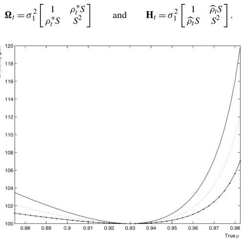
Theorem 1 says that the conditional variance of every opti-mized portfolio will be greater than or equal to the conditional variance of the portfolio optimized on the true covariance ma-trix. It is important to note that this will be true for any vector of expected returns and any required excess return. Correct co-variance information will allow the investor to achieve lower volatility, higher return, or both. We will typically measure this in terms of the increase in required return, holding volatility constant. The magnitude of these gains will depend on the re-turns expected by the investor. To better explain this idea, we report a graphical example in Figure 1. In this figure the esti-mated correlation is .93, but the true correlation may be differ-ent. For an investor who takes the expected returns on stocks to be three times the return on bonds, the gain ranges from 0% to 20% depending on the ratio of the variances and the true cor-relation. As is clear, the efficiency loss in very high when the true value of the correlation is close to unity. The picture also shows the content of the theorem through a graphical argument: The loss function is minimized when the estimated correlation is equal to the correct correlation.
Theorem 1 also suggests that there is always a pair of ex-pected returns that delivers acostless mistake. An immediate implication of this finding involving the Sharpe ratios is a bi-variate allocation problem, which can be shown by the follow-ing corollary.
Corollary 1(A costless mistake). If the two assets involved in a bivariate asset allocation problem have the same Sharpe ratio when measured by bothandH, then there is no loss of efficiency.
Proof. LetSdenote the ratio σ2
σ1, and letρt be the estimated
correlation and ρt∗ be the true correlation. Then the matrices tandHtcan be written as
t=σ12
1 ρt∗S
ρt∗S S2
and Ht=σ12
1 ρtS
ρtS S2
.
Figure 1. Two Assets’ Example of Efficiency Loss as a Function of the True Correlation for Different Volatilities’ Ratios ( σ1/σ2=1.5; σ1/σ2=1; σ1/σ2=.5). The estimatedρis .93. The ratio of
ex-pected returns is 3.
The matrixtH−t1has eigenvalues
ρt∗−1 ρt−1 and
ρt∗+1
ρt+1 with
corre-sponding eigenvectors[ −1S 1]and[1 S]. Use Theorem 1
to conclude the proof.
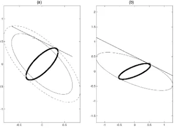
This result is illustrated graphically in Figure 2. The axes measure the investment in each asset, and the ellipses are loci of the constant volatility. One ellipse corresponds to the truth, and the other is the false ellipse. The required return in (2) is a straight line, so that the solution is a tangency. Clearly the ac-tual variance of the portfolio using the true ellipse is lower than using the false ellipse. The ill-informed investor will choose the square point for his or her portfolio whereas the well-informed investor will select the circle, thus obtaining a lower volatility. Figure 2(b) illustrates the situation described in Corollary 1.
The vector of expected returns that we have assumed is not required to also be the true one. This will prompt our investi-gation over a wide range of alternatives forµ. This also reveals that selecting the best covariance matrix estimator based on a Sharpe ratio criterion may be misleading. We summarize this finding in the following proposition and its corollary.
Proposition 1. LetHand be the estimated and true co-variance matrices, and letwandw∗be the associated optimal
portfolio weights computed according to (2). Then there always exists a vector of true expected returnsχsuch that
w′χ
√
w′w≥
w∗′χ
√
w∗′w∗. (5)
Proof. By construction, (w−w∗)′µ=0. Because µ>0, there exists at least one element i of w and w∗ such that
wi−w∗i >0. Therefore, it is always possible to offset any
dif-ference in the denominators of (6) by makingw′χ much larger thanw∗′χby selecting a large enoughith entry ofχ.
Corollary 2. Let χ =T1
T
t=1rt and = T1Tt=1rtr′t and
define the empirical Sharpe ratio as the one computed using χand. Then the empirical Sharpe ratio can select either port-folio regardless of the true expected returns,
w′χ
√
w′w
w∗′χ
√
w∗′w∗. (6)
Proof. Follows directly from Proposition 1.
Several authors have proposed measures of the value of time-varying covariance matrices based on a Sharpe ratio criterion. The fact that this method can potentially lead to the selection of the wrong covariance estimator motivates our quest for an alternative measure. Ideally, this measure should be able to pick the correct estimator independently of the model of expected returns.
2.1 Expected Returns
Different investors at different times will have different vec-tors of expected excess returns. Thus we calculate the efficiency gain for all possible vectors of expected returns. In a bivariate problem, these can be expressed as a pair of numbers or, in po-lar coordinates, as a length and an angle. From (3) and (4), it is clear that the relative volatilities do not depend on the length of the vector of expected returns, but they do depend on the
(a) (b)
Figure 2. Loss of Efficiency. (a) The case in which the variances of the two assets are correctly estimated, but a correlation of−.75 is assumed instead of the true of .7. (b) The costless mistake case. [ min variance frontier (correct); min variance frontier (estimated); required return;
optimal portfolio (correct); optimal portfolio estimated; efficiency loss.]
angle. Thus it is sufficient to consider one dimension of ex-pected returns. In the empirical section we consider 11 pairs of expected returnsµ= [sinπ20j,cos20πj], forj∈ {0, . . . ,10}. The endpoints correspond to hedging problems where one asset is held for return and the other is held for a hedge. Whenj=5, expected returns are equal, and the solution is the minimum variance portfolio.
2.2 Bayesian Priors
We also summarize our results adopting a quasi-Bayesian perspective, attaching prior probabilities to the vectors of ex-pected returns. Obtaining priors for our vectors of exex-pected re-turns is not an easy task and certainly is a subject of debate in the literature. In the context of the two bivariate portfolio appli-cations that we analyze in Section 5, we consider our approach as a way of specifying priors that formalize the idea that on av-erage, stocks should deliver a higher return than bonds and that the S&P500 and the NASDAQ should have approximatively the same expected returns. This is in the spirit of the analy-sis of Ibbotson and Sinquefield (1989). We regard what follows as a way of summarizing our results; an investor with differ-ent views may choose an alternative vector of prior probabili-ties. More precisely, we construct priors in the following way. For a given sample of returns,rt= [r1,t,r2,t],t=1, . . . ,T, we
take sample averages over the maximum number of nonoverlap-ping consecutive subsamples of lengthN. This gives a sample of realized meansµn= [µ1,n, µ2,n],n=1, . . . ,T/N. However,
for this sample to be a proxy of expected returns, it must be the case that µn≥0,∀n. Following Fleming et al. (2001),
we discard the pairs for which at least one of the elements is negative. This leads us to discard 42 out of 66 pairs for the stocks and bonds case and 18 out of 42 pairs for the stocks and
stocks case analyzed in Section 5. In both cases we take av-erages over 6 months. For the remainingNpairs, we compute
θn=π2arctan(µµ1,n
2,n), solving the system
µ1,n=ksin
π
2θn ,
µ2,n=kcos
π
2θn ,
∀n=1, . . . ,N. Asθ∈ [0,1], we find the parametersa andb
that maximize the log-likelihood function of a beta distribution,
(a,b)=arg max log
a,b
L(θ1, . . . , θN;a,b)
=arg max
a,b
Nlog
1 1
0 ta−1(1−t)b−1dt
+(a−1)
N
i=1
log(θi)+(b−1)
N
i=1
log(1−θi).
Finally, we compute the prior probability associated with each of the aforementioned pairs using the maximum likelihood es-timators (MLEs)aandb,
Pr(θ=θj)=
1
ϒ
θja−1(1−θj)b−1
1
0ta−1(1−t)b−1dt ,
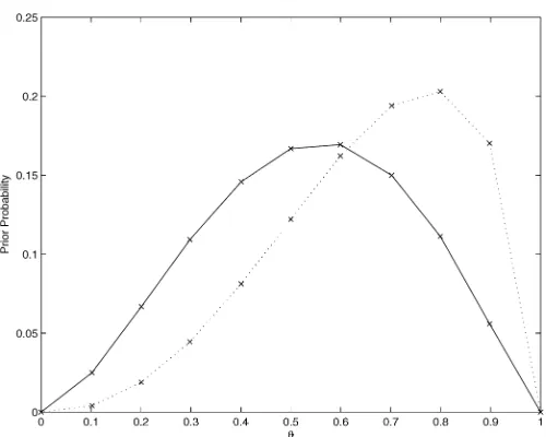
whereϒ normalizes probabilities so that they sum to 1. In the empirical section we discuss two main examples involving the bivariate asset allocation problem between stocks and bonds and between the Dow Jones and the S&P500. The empirically estimated priors for these two pairs of assets are shown in Fig-ure 3.
Figure 3. Priors for the Distribution of Expected Returns ( Bonds-SP; Dow-SP). The horizontal axis reportsθ, which is equal to arctan(µSP/µbonds) and arctan(µDow/µSP) for the stocks-bonds and the stocks-stocks allocations. As θ increases, the expected return of stocks goes up relative to bonds and the expected return of the Dow increases with respect to SP.
3. TESTS
In this section we present the tests that we implement later in the empirical analysis. The first strategy relies on Theorem 1, the second tests the accuracy of a method, and the third aims to test the equality of two models.
3.1 Comparison of Volatilities
A portfolio constructed to optimize (1) assuming an arbi-trary vector of expected excess returns will have standard de-viationσt∗defined as in (4). From Theorem 1, we have that
E
Therefore, Theorem 1 offers a strategy for comparing co-variance matrices, based on the idea of choosing coco-variance matrices that achieve lowest portfolio variance for all relevant expected returns. To benefit fully from the content of this theo-rem, we need to show that, at least asymptotically, we can ob-tain the conditional covariance matrix without knowing the true conditional mean forecast of returns. The following theorems show that by considering returns whose unconditional sample mean has been subtracted, we obtain a consistent estimator of the true portfolio variance.
Theorem 2. LetHtandtbe the estimated and true
covari-ance matrices. Also, let r be the in sample mean of rt, and
letµ andχ be the constant hypothetical and true conditional means ofrt. Optimal portfolio weights,wtare defined as in (2)
and are assumed to be weakly stationary and bounded. Then
plim
Proof. Rewrite the left side of (7) as
0≤plim
where the inequality is implied by the absolute value. Because squared portfolio returns are scalars, we can take the trace of (8) and rearrange terms to get
≤plim
and the inequality follows again from the absolute value. Clearly,
plim(r−χ)=0 and plim(rr′−χ χ′)=0,
which combined with (8) and (9), concludes the proof.
Theorem 2 relies on the assumption that the true conditional expected value of returns is constant. When the time interval is small, this assumption is not very strong. Given that the focus of this article is on agents that have a 1-day investment hori-zon, we can expect forecasts of returns to be characterized by a small variation around the constant value that we assumed in Theorem 2. As the sampling interval shrinks, we can expect variances and covariance to become smaller as well. We for-malize these ideas in the following theorem.
Theorem 3. Define Ht,t,r,µ, andwt as in Theorem 2, ranging terms, (10) implies that
0≤ lim
Using the properties of the absolute value operator and
Theo-where the second line follows from the definition of χt = E(t−1)rt. Denoteεt=rt−Et−1rtand note that
finite. Also note, that the law of iterated expectations implies that
E(w′tεtδ′twt)(wt′+jδt+jε′t+jwt+j)
=0, ∀j≥1. (15)
By the law of large numbers, it follows from (13)–(15) that
plim
Combining (11), (12), (16), and (17) concludes the proof.
3.2 Testing the Accuracy of a Method
For any vector of expected returns, we can test whether the portfolio variance divided by the predicted variance has a condi-tional mean of 1. This amounts to estimatingβin the regression
(w′trt)2
w′tHtwt −
1=Xtβ+εt, (18)
whereXt can be chosen to include an intercept, a lagged
de-pendent variable, and some dummies for predictions that the variance is in the bottom part or the top part of the distribution. These dummies should help us understand whether the estima-tor is unbiased when the variance takes on very extreme values. The null of the test isH0:β=0.
3.3 Testing the Equality of Two Models
Suppose that we have two different time series of covariance matrices{Hjt}2j
=1and a set{µk}Kk=1of hypothesized vectors of expected returns divided by the required excess return µ0. In each period a set of portfolio weights is constructed based on a covariance matrix and an expected return. Denote this bywjt,k, and denote the portfolio return by
πtj,k=(wtj,k)′(rt−r), (19)
wherewjt,k= (H j t)−1µk
(µk)′(Hjt)−1(µk)
. Now construct the squared return
on this portfolio and subtract it from the squared return on the second portfolio,
utk=(πt1,k)2−(πt2,k)2, t=1, . . . ,T. (20) The null hypothesis is that the mean ofuis 0 for all k. We ignore the problem of parameter estimation in this article, al-though there is now a large literature extending Diebold and Mariano–style tests to many different environments (see, e.g., West and Cho 1995; West 1996; West and McCracken 1998).
The Diebold–Mariano testwould examine each u time se-ries separately. By regressing on a constant and using aNewey– West covariance matrix, the null of equal variance is simply a test that the mean ofuis 0. In principle, the covariance matrix should correct the size of the test for heteroscedasticity, auto-correlation, and nonnormality all at once.
The test could be more powerful if there were not so much heteroscedasticity, however. Suppose that the returns were mul-tivariate normal. Then the expectation of squared portfolio re-turns and the variance of squared portfolio rere-turns would be given by
E(w′rt)2=w′w (21)
and
var[(w′rt)2] =2[w′w]2=2[µ′−1µ]−2. (22)
Hence dividing u by its standard deviation could improve the efficiency with which the mean is estimated. Because the true covariance matrix is unknown and two estimators are be-ing compared, a natural adjustment is the geometric mean of the two variance estimators,
vkt =ukt2(µk′(H1t)−1µk)(µk′(H2t)−1µk)1/2. (23) This transformation does not change the null or alternative hypothesis, because the factor in square brackets is predeter-mined and positive. It should simply improve the sampling properties of the test. If these are not sufficiently accurate to makevan iid series, then it too must be tested with a robust co-variance matrix. Hence we should apply the Diebold–Mariano test to each of thevseries as well to theuseries. To test whether covariance methods 1 and 2 are equal, we should do a joint test for allk. Let
then use generalized method of moments (GMM) with a vector heteroscedasticity and autocorrelation consistent (HAC) covari-ance matrix to estimate
Ut=βuι+εu,t (26)
and
Vt=βvι+εv,t, (27)
whereιis ak×1 vector andβu andβv are scalars. We then
have that
T1/2G−u1/2U→N(βuι,Ik)
and
T1/2G−v1/2V→N(βvι,Ik),
whereGuandGvare the estimated robust covariance matrices
taking into account the serial correlation and heteroscedasticity of the residuals of (26) and (27) and
U= 1
T
T
t=1 Ut
and
V= 1
T
T
t=1 Vt.
Under the null,βuandβvare both equal to 0. If the null
hypoth-esis is rejected, then we can examine how it is rejected.
4. ESTIMATORS
The literature details several approaches to estimating condi-tional covariance matrices. In this article we focus on five alter-native models; we briefly discuss these models in this section, and provide details in the Appendix. A simple approach for es-timating multivariate models is orthogonal generalized autore-gressive conditional heteroscedasticity (GARCH) (Alexander 2000). The procedure relies on the construction of uncondition-ally uncorrelated linear combinations of the series of returns. Then, assuming that the conditional correlations are all 0, it is possible to construct the whole covariance matrix estimating univariate GARCH models for some or all of these.
Multivariate GARCH is an alternative and more general ap-proach to the problem. The vec model, introduced by Engle and Kroner (1995), is the most general expression of this class of models. Letting vec(Ht)denote the vector of all covariances
and variances, the parameterization for the first-order case can be expressed as
vec(Ht)=vec()+Avec(rt−1r′t−1)+Bvec(Ht−1), (28) where much of the structure ofAandB, bothn2×n2 matri-ces, comes from the symmetry of the covariance matrix. This model does not guarantee the positive definiteness of the ma-trixHwithout additional restrictions. Furthermore, even after imposing the restrictions implied by the symmetry, the number of parameters to be estimated is very large and equal ton(n2+1)+
2(n(n2+1))2. The Baba, Engle, Kraft, and Kroner (BEKK) repre-sentation as discussed by Engle and Kroner (1995) and Engle
(2002) can provide useful restrictions to (28). The first-order case can be written as
Ht=+A(rt−1r′t−1)A′+BHt−1B′. (29) In this article we consider two special cases where theAandB matrices are scalar and diagonal; details are reported in the Ap-pendix. More highly parameterized models can be found in the literature (see, e.g., Engle and Kroner 1995; Bollerslev, Engle, and Nelson 1994; Engle and Merzich 1996). The estimator ap-plied in this article is subject to the constraint that the long-run covariance matrix is the sample covariance matrix (see Engle and Merzich 1996). This approach differs from the MLE only in finite samples, but it often gives improved performance and reduces the number of parameters to be estimated. Using this constraint, in the scalar BEKK the intercept is simply
=(1−α−β)S, whereS=1
T
T
t=1
(rtr′t). (30)
The DCC model is a new type of multivariate GARCH that is particularly convenient for big systems. The DCC method first estimates volatilities for each asset and computes the standard-ized residuals. It then estimates the covariances between these using a maximum likelihood criterion and one of several mod-els for the correlations. The correlation matrix is guaranteed to be positive definite. In the article we use two alternative ver-sions of DCC. The first version is the standard DCC with mean reversion (henceforth DCC–MR), discussed by Engle (2002). The second one is asymmetric DCC (henceforth Asy-DCC), introduced by Cappiello et al. (2003). The two specifications differ for an additional term in Asy-DCC that allows correla-tion to increase more when both returns are falling than when they are both rising. We also model the asymmetric impact of news on individual asset variances (as in Engle and Ng 1993) in the first step in estimating the Asy-DCC model in the empirical section. Details are reported in the Appendix.
5. STOCKS AND BONDS
5.1 Model Estimates
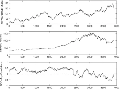
In this section we present the results of the proposed testing strategies applied to an example using daily data from S&P500 and 10-year bond futures (source, DataStream; code names, are CTYCS00 and ISPCS00). These are continuous series of fu-tures settlement prices, starting at the nearest contract month, which form the values for the continuous series until either the contract reaches its expiration date or until the first business day of the actual contract month. At this point, the next contract month is taken. The Treasury Bond has a quarterly trading cy-cle, whereas the S&P500 has a monthly trading cycle. Returns are computed as the difference of the logarithm of prices on two consecutive days. The sample period is 8/26/1988–8/26/2003. Figure 4 shows the time series of these two series. It also shows the dynamic correlations estimated using the Asy-DCC model. It is interesting to note that for more than half of the sample, he two series were positively correlated, whereas over the past few years, correlation has been mostly negative.
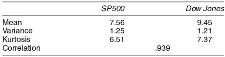
It is worth taking a look at some descriptive statistics. Ta-bles 1 and 2 show that the annualized return on stocks has been
Figure 4. Time Series of S&P500 Futures and 10-Year Bonds Fu-tures. The sample period is 8/26/88–8/26/03. The period of negative correlation begins around year 2000.
about four times the return on bonds. Because the series are fu-tures, these can be interpreted as excess returns. A much higher volatility on stocks is the reasonable counterpart to the previ-ous finding. Interestingly, the average correlation has been very close to zero on average. Next we estimate the models described in Section 4. The results are also reported in Tables 1 and 2. There is evidence of asymmetry in the stocks’ variance, but the same cannot be argued for bonds. It can also be appreciated that the variances of stocks and bonds are almost equally persistent. Before moving to the tests, we need to specify the priors associated with the vectors of expected returns. We follow the strategy reported in Section 3 and construct a sample of 3-month averages of stocks and bonds returns. We then fit a beta distribution on the nonnegative pairs and use the estimated coefficients to associate priors with the hypothetical expected returns based on the polar coordinates. Figure 3 plots these pri-ors. The distribution looks fairly reasonable, because a higher probability is attached to pairs in which the expected return on bonds is relatively lower than the expected return on stocks. Figure 3 also reports priors for the case in which the asset allo-cation experiment involves S&P500 and Dow, which we discuss in detail in the next section. Clearly, this distribution looks sym-metrical, with the highest probability associated with the case in which the two expected returns are about the same.
5.2 Volatility Ratios
Having estimated the coefficients of the model, we can run the tests proposed in Section 3. Table 3 reports the results for the in-sample estimates. The best (i.e., lowest) standard devi-ation for each pair of expected returns has been normalized
Table 1. Sample Statistics (stocks and bonds)
Stock Bond
Mean 8.64 1.98
Variance 1.16 .149
Kurtosis 17.2 6.15
Correlation .061
NOTE: The means have been annualized.
to 100. A number like 105 in the tables can be interpreted, using formulas (3) and (4), as a 5% higher return than might have been required had we known the true covariance matrix. Hence if we have a target return of 10% by using the wrong covariance matrix, then, using the true one, we can achieve the same portfolio variance, but requiring a return of 10.5%. The first thing to notice is that the DCC models are always the best compared with a constant estimator. The differences are not too great, but this can be explained using the argument that the value of the correlation information is usually higher for highly positively correlated assets, which is not the case for stocks and bonds. Another interesting finding is that Asy-DCC seems to perform better for the expected returns that are more likely to be the true ones. Indeed, averaging sample standard deviations using the weighting scheme suggested by the priors shows that Asy-DCC delivers the lowest value. The difference between the two versions of DCC do not seem to be significant on average.
5.3 Bivariate Tests at Each Expected Return
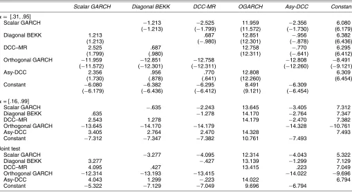
The Diebold–Mariano approach to test differences between estimators at each vector of expected returns would offer the possibility to compare the various approaches at 11 different expected returns. Instead of reporting the results for all vectors ofµ, we focus on those expected returns whose ratios are closer to the ratio of true unconditional averages of stocks and bonds in the sample that we are considering. Tables 1 and 2 show that the relevant ratios should be around 4. Therefore, we consider µ= [.31;.95]andµ= [.16;.99], where the first number is rel-ative to bonds. The results are given in Table 4. The top panel reports both the unweighted and the weighted versions of the test, whereas in the bottom two panels the test is implemented by correcting the squared differences as suggested in the pre-vious section. The null hypothesis is that there is no difference between the models, whereas the alternative is that the model in the row is better than that one in the column.
If differences are not always significant for µ= [.31;.95], when the expectation on stocks’ returns is slightly increased relative to bonds, then this version of DCC always becomes strongly significant. The top panel of Table 4 also shows that adjusting for the geometric mean of the two variance estimators appears to be helpful. In at least four more cases we can say that two models are significantly different at 5% level, where the unweighted version of the model failed to do so.
5.4 Joint Tests
Using the time series of estimated conditional covariance matrices and constructing weights as explained in Section 2, implementing the Diebold–Mariano strategy in its joint ver-sion is straightforward. All that is needed is to stackukt,∀k=
1, . . . ,11, callUtthe resulting vector, and use GMM with
vec-tor HAC covariance to estimateβ in
Ut=βι+εt. (31)
The null hypothesis would beβ=0. The numbers reported in Table 4 aret-tests on the estimatedβof (31), whereUtis
con-structed as the difference of the squared realized returns of the
Table 2. Parameter Estimates (stocks and bonds)
Stock variance parameters Bond variance parameters Correlation parameters Models ω1 α1 β1 γ1 ω2 α2 β2 γ2 ω12 θ1 θ2 θ3
Multivariate GARCH .024 .057 .918 .004 .057 .918 .003 (.001) (.005) (.001) (.000) (.005) (.001) (.000)
Diagonal BEKK .158 .983 .185 .981
(.006) (.002) (.006) (.001)
Orthogonal GARCH .005 .043 .954 .002 .027 .958 .553
(.001) (.003) (.003) (.000) (.003) (.005) (.028)
DCC–MR .006 .044 .95 .002 .027 .958 .022 .973
(.001) (.003) (.004) (.000) (.003) (.005) (.003) (.003)
Asy-DCC .019 .001 .923 .123 .002 .024 .958 .005 .024 .972 −.002
(.002) (.005) (.006) (.008) (.000) (.004) (.005) (.005) (.003) (.003) (.005)
NOTE: Returns have been multiplied by 100 to improve the numerical performance of the estimation routine. The numbers in parentheses are standard errors.
Table 3. Comparison of Volatilities (stocks and bonds)
µbonds µstocks Scalar GARCH Diagonal BEKK DCC–MR Orthogonal GARCH Asy-DCC Constant
1.00 0 100.772 100.107 100.000 103.681 100.211 106.565
.99 .16 100.768 100.105 100.000 103.472 100.196 105.357
.95 .31 100.736 100.096 100.000 103.447 100.148 104.149
.89 .45 100.671 100.075 100.000 103.707 100.059 102.997
.81 .59 100.640 100.107 100.068 104.544 100.000 102.119
.71 .71 100.648 100.173 100.189 106.404 100.000 101.817
.59 .81 100.572 100.131 100.202 110.003 100.000 102.462
.45 .89 100.465 100.057 100.095 116.929 100.000 104.535
.31 .95 100.705 100.341 100.222 131.308 100.000 108.038
.16 .99 100.141 100.986 100.822 166.795 100.000 110.800
0 1.00 100.737 100.329 100.152 126.545 100.000 106.510
Overall (weighted) 100.727 100.362 100.309 128.795 100.000 106.107
NOTE: Sample standard deviations of minimum variance portfolios subject to a required return of 1. Each row of the table reports the results for the pair of expected returns of the corresponding two columns. The lowest standard deviation is normalized to 100, so that a number like 105 means that knowing the true covariance matrix, a 5% higher return could be required. The last row of the table averages the standard deviations of the model in the corresponding column using the priors as weighting factors.
Table 4. Diebold and Mariano Test (stocks and bonds)
Scalar GARCH Diagonal BEKK DCC-MR OGARCH Asy-DCC Constant
µ= [.31, .95]
Scalar GARCH −1.213 −2.525 11.959 −2.356 6.080
(−1.213) (−1.799) (11.572) (−1.730) (6.179)
Diagonal BEKK 1.213 .687 12.851 −.956 6.382
(1.213) (−.980) (12.301) (−.878) (6.436)
DCC–MR 2.525 .687 12.758 −.770 6.295
(1.799) (.980) (12.311) (−.641) (6.412)
Orthogonal GARCH −11.959 −12.851 −12.758 −12.808 −8.491
(−11.572) (−12.301) (−12.311) (−12.260) (−9.121)
Asy-DCC 2.356 .956 .770 12.808 6.309
(1.730) (.878) (.641) (12.260) (6.454)
Constant −6.080 −6.382 −6.295 8.491 −6.309
(−6.179) (−6.436) (−6.412) (9.121) (−6.454) µ= [.16, .99]
Scalar GARCH −.635 −2.243 13.645 −3.405 7.312
Diagonal BEKK .635 −1.278 14.170 −2.764 7.347
DCC–MR 2.543 1.278 14.179 −2.470 7.382
Orthogonal GARCH −13.645 −14.170 −14.179 −14.328 −10.761
Asy-DCC 3.405 2.764 2.470 14.328 7.493
Constant −7.312 −7.347 −7.382 10.761 −7.493
Joint test
Scalar GARCH −3.277 −4.095 12.314 −4.043 5.322
Diagonal BEKK 3.277 −.427 13.139 −1.299 7.129
DCC–MR 4.095 .427 13.415 .223 7.049
Orthogonal GARCH −12.314 −13.193 −13.415 −14.022 −9.696
Asy-DCC 4.043 1.299 −.223 14.022 6.794
Constant −5.322 −7.129 −7.049 9.696 −6.794
NOTE: The top panel reports thet-statistics for the Diebold and Mariano test when the vector of expected returns isµ=[.31, .95]. The numbers in brackets refer to the unweighted version of the test, whereas the other results are weighted as described in the text. The middle panel gives the results of the weighted Diebold and Mariano test when the vector of expected returns is
µ=[.16, .99]. The bottom panel reports the results of the joint (i.e., all of the assumed vectors of expected returns are taken into account) weighted test. A positive number means that the row is better than the column.
corresponding method in the column and the one in the row. Therefore, a negative number is evidence in favor of better per-formance of the column method in a pairwise comparison.
Were we to weight the differences of the squared returns by the standard deviations as suggested in (23), we would expect to be able to get more rejections than in the unweighted case. Ta-ble 4 shows that with this weighting, Asy-DCC performs better than most of the alternative estimators, although the difference is not always significant. The only estimator that Asy-DCC is not able to clearly outscore is DCC–MR. This means that al-though the asymmetric components of variance and correlation help reduce sample standard deviation, they fail to do so in a significant way.
5.5 Valuing Correlations by Simulation
One way to assess the ability of the proposed strategies to value correlation information is to simulate a time series of returns using the estimated parameters of one of the models discussed before, apply the proposed tests, and check whether (and if so, how much) the alternative estimators differ from the simulated truth. The results reported in the previous sec-tions showed that among the dynamic estimators, the two DCC models seemed to perform better. In particular, the Asy-DCC slightly outperformed the symmetric DCC. Therefore, in this section we simulate 10,000 observations from an Asy-DCC model, using the values of the parameters reported in Tables 1 and 2. In a first stage we let both variances and correla-tions be time-varying, whereas in a second simulation we keep variances constant at their unconditional average and let just the correlations be dynamic. In principle, the second approach should be able to say more about the value of correlation infor-mation alone.
Because our results so far do not indicate a great differ-ence among the alternative dynamic models, in this section we focus on a direct comparison between a time-varying covari-ance model and the constant unconditional estimator. Table 5 gives the results of the volatility ratios approach for the case where the whole simulated covariance matrix is time-varying. As pointed out earlier, these numbers can be equivalently inter-preted as the increase in required return that can be achieved
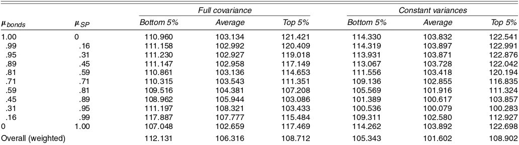
with no change in volatility using the covariance information. Because the Asy-DCC, being the true data-generating process, always performs better than the constant estimator, we report only the constant estimators in the tables of this section. We also report the gains computed on the subsample in which the correlations fall into the bottom and the top 5% percentiles. This leads to a strategy in which we adjust our portfolio only when the forecasted value of correlation is very high or very low.
As already argued, the value of correlation information can be very important when correlation itself becomes extreme. Ta-ble 5 shows that the knowledge of the right covariance matrix in these days can be as high as 22%. The same analysis is repeated for simulating series, whose variances are constant at the true unconditional value of stocks and bonds and assuming that the correlation process is still Asy-DCC. The results, given in the last three columns of Table 5, seem to reinforce the outcome of the previous simulation. An interesting finding is that when the ratio of expected returns is close to the ratio of true uncondi-tional averages of stocks and bonds, there appears to be almost no loss. This is the case of acostless mistake, which has been shown to occur whenever the two assets have the same Sharpe ratio.
5.6 A Small-Sample Monte Carlo Experiment
The theorem on which we base our tests gives large-sample results. In this section we explore the significance of the pro-posed methods on a small sample and evaluate how results change as we increase the length of the time series. Again we choose to simulate data from an Asy-DCC model, and again we first let the whole covariance matrix be time-varying and then hold variances constant. We start the analysis by simulating 100 samples of 500 observations and estimating all the models on this dataset. We then allocate assets according to (2) and run the joint Diebold–Mariano test (from now on we always refer to the weighted version of the test) in each Monte Carlo trial. Table 6 gives the results. The numbers reported in this table are the times that the method in the row results in a significantly smaller sample standard deviation than the model in the cor-responding column, using a 5% significance level. Clearly, in small samples this strategy does not seem to have much power
Table 5. Importance of Extreme Correlations (stocks and bonds)
Full covariance Constant variances
µbonds µSP Bottom 5% Average Top 5% Bottom 5% Average Top 5%
1.00 0 110.960 103.134 121.421 114.330 103.832 122.541
.99 .16 111.158 102.992 120.409 114.319 103.897 122.991
.95 .31 111.230 102.927 119.018 113.931 103.871 122.876
.89 .45 111.147 102.958 117.149 113.067 103.728 122.042
.81 .59 110.861 103.136 114.653 111.556 103.418 120.194
.71 .71 110.315 103.543 111.351 109.136 102.855 116.835
.59 .81 109.516 104.381 107.208 105.569 101.916 111.324
.45 .89 108.962 105.944 103.086 101.389 100.617 103.857
.31 .95 111.197 108.321 103.433 100.536 100.079 100.283
.16 .99 117.887 107.777 115.484 109.311 102.580 112.927
0 1.00 107.048 102.659 117.469 114.262 103.892 122.698
Overall (weighted) 112.131 106.316 108.712 105.343 101.602 108.902
NOTE: The results reported under “Full covariance” are obtained from simulations of the full covariance matrix using the Asy-DCC estimated parameters of the bivariate stocks and bonds distribution. “Constant variances” means that only the dynamic correlations were simulated, while variances were kept constant at their unconditional value. The “Bottom 5%” and “Top 5%” refer to the percentiles of the distribution of conditional correlation. The numbers reported are the extra return that an investor using Asy-DCC could have required compared with an investor using constant unconditional estimators, when correlation takes on extreme values.
Table 6. Small-Sample Monte Carlo for Simulated Stocks and Bonds
T Scalar GARCH Diagonal BEKK DCC–MR Asy-DCC Constant
Full covariance
500 Scalar GARCH 0 0 0 14
Diagonal BEKK 42 0 2 36
DCC–MR 54 16 4 52
Asy-DCC 38 9 0 40
Constant 0 0 0 1
100.979 100.259 100.039 100.000 102.384
1,000 Scalar GARCH 0 0 0 42
Diagonal BEKK 76 0 1 69
DCC–MR 85 20 0 82
Asy-DCC 75 24 1 71
Constant 0 0 0 0
101.192 100.480 100.275 100.000 104.031
5,000 Scalar GARCH 0 0 0 100
Diagonal BEKK 100 0 0 100
DCC–MR 100 58 0 100
Asy-DCC 100 96 30 100
Constant 0 0 0 0
100.929 100.554 100.443 100.000 104.956
Constant variances
500 Scalar GARCH 2 0 12 9
Diagonal BEKK 8 2 8 9
DCC–MR 23 8 28 24
Asy-DCC 23 15 1 29
Constant 4 2 0 17
100.481 100.406 100.000 100.319 100.598
1,000 Scalar GARCH 6 0 1 11
Diagonal BEKK 9 0 0 10
DCC–MR 48 34 9 47
Asy-DCC 57 38 0 60
Constant 14 6 0 7
100.507 100.305 100.000 100.168 100.621
5,000 Scalar GARCH 0 0 0 54
Diagonal BEKK 54 0 0 66
DCC–MR 100 96 0 100
Asy-DCC 100 94 0 100
Constant 2 0 0 0
100.550 100.209 100.000 100.033 100.874
NOTE: The series were simulated assuming an Asy-DCC distribution with parameters estimated from the stocks and bonds joint distribution. The top panel assumes that the whole covariance matrix is time varying, while in the bottom panel variances are held constant. The number of simulations increases from 500 to 5,000. The numbers reported in the tables represent the number of times (out of 100 Monte Carlo trials) that the estimator in the row produced a significantly smaller sample variance than the model in the column. The joint Diebold and Mariano test was used to run the comparison between each pair of models. The last line of each panel reports the comparison of average (weighting expected returns according to the prior) volatilities for each method.
for choosing the best covariance estimator. The comparison be-tween the two DCC estimators results in a tie, whereas in about half of the trials the two DCC models perform better than the competitors. The situation clearly changes as we increase the length of the simulation. At 1,000 observations, the two DCC estimators achieve a significantly lower variance in almost 80% of the trials when the entire covariance matrix is time-varying and in 50% of the trials when we keep the variance fixed. Both results are about twice as great the respective results at 500 sim-ulations. A total of 5,000 observations seems to be sufficient to invoke the large-sample results. When variances and correla-tions are dynamic, the true model is significantly better than the DCC–MR 30% of the time, but when only correlations are varying, this number drops to 0. This suggests that the 30% re-sult is due mainly to the asymmetric component in the variance process.
6. OTHER DATASETS
6.1 Dow Jones and S&P500
Figure 1 showed that the efficiency loss increases as the cor-relation of the two assets becomes close to 1. In the previous
sections we showed that the unconditional correlation between stocks and bonds was almost zero in the sample that we consid-ered. Indeed, the analysis on simulated data also pointed toward significant but very small differences in terms of efficiency be-tween conditional and unconditional estimators. One possibil-ity would be to consider a portfolio composed of two assets that are highly correlated. Using data from Yahoo! Finance starting on 2/4/1993 sand ending on 7/22/2003, we implement the same strategy of Section 5 on S&P500 and Dow Jones Industrials. Tables 7 and 8 reports some summary statistics along with the estimates of the models that we consider.
The two assets appear to have similar sample mean and stan-dard deviation, and the average correlation is now extremely
Table 7. Sample Statistics (S&P500 and Dow)
SP500 Dow Jones
Mean 7.56 9.45
Variance 1.25 1.21
Kurtosis 6.51 7.37
Correlation .939
NOTE: The means have been annualized.
Table 8. Parameter Estimates (S&P500 and Dow)
S&P500 variance parameters Dow Jones variance parameters Correlation parameters Models ω1 α1 β1 γ1 ω2 α2 β2 γ2 ω12 θ1 θ2 θ3
Multivariate GARCH .038 .292 .934 .041 .292 .934 .037 (.002) (.008) (.002) (.002) (.008) (.002) (.002)
Diagonal BEKK .220 .973 .223 .971
(.007) (.002) (.007) (.002)
Orthogonal GARCH .005 .066 .932 .003 .088 .892 .953
(.001) (.006) (.006) (.001) (.007) (.010) (.006)
DCC–MR .005 .066 .932 .009 .082 .914 .042 .955
(.001) (.006) (.006) (.002) (.006) (.007) (.005) (.005)
Asy-DCC .012 .001 .923 .141 .016 .017 .914 .121 .053 .938 .004
(.002) (.008) (.007) (.011) (.002) (.010) (.008) (.011) (.006) (.007) (.005)
NOTE: Returns have been multiplied by 100 to improve the numerical performance of the estimation routine. The numbers in parentheses are standard errors.
high: .939. The asymmetric component is an important factor in both variance processes but apparently is not too relevant for the dynamics of the correlation. Figure 3 shows the priors that we attach to the 11 pairs of hypothetical expected returns. In this case the distribution is more symmetrical than that of stocks and bonds.
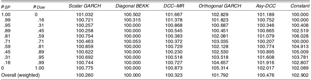
The volatility ratios in Table 9 do not seem to show a great difference between the proposed estimators. The diagonal BEKK is usually the best method, but in some cases (especially those closer to the true ratio of sample means) the gap does not appear significant. The results from the weighted Diebold– Mariano joint test in Table 10 confirm these findings. The only model that the diagonal BEKK cannot outscore at 5% signif-icance level is Asy-DCC. We also use the weighted Diebold– Mariano univariate test. Because the true ratio of mean re-turns is around 1.25, we implement this test forµ= [.59;.81]. The numbers of rejections of the three leading models remain almost unchanged, although the negativet-statistics in the Asy-DCC column provide evidence of this model’s good perfor-mance.
We now turn to the value of correlation information. As-suming that Asy-DCC is the data-generating process, we cre-ate 10,000 observations again using the double approach of first simulating both variances and correlations as time-varying and then assuming that the variances are constant and only the correlations are dynamic. Table 11 shows that when the full co-variance matrix is simulated, the loss of efficiency is higher on average than in the case of simulated stocks and bonds. This is
a result of the higher sensibility of the volatility ratio for high values of correlations. If we consider the extreme values of cor-relation, then we end up with losses varying from 8% to 37% in the top percentile and from 6% to 30% in the bottom percentile. Table 11 reports also the results of the simulation involving only time-varying correlations. The loss of efficiency is around 20% in the extremes of the distribution with peaks of more than 30% and around 10% on average. Again, note the costless mistake occurring atµ=[.71; .71].
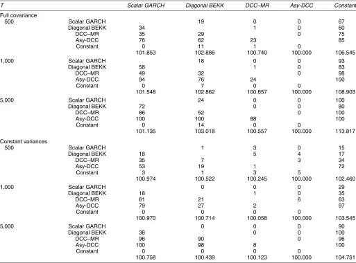
We conclude this section with a small-sample Monte Carlo in the same spirit of that discussed in Section 5 for the stocks and bonds asset allocation case. The data-generating process is the Asy-DCC model with the coefficients reported in Tables 7 and 8. When the entire covariance matrix is time-varying, the Diebold–Mariano test seems to have sufficient power to find the best estimator also in the smallest sample of 500 obser-vations, whereas when only the correlation is allowed to vary, the two DCC models are almost undistinguishable even in large samples. This indicates that the asymmetric component of the variances role in determining the performance of an estimator. However, an average gain of about 4% can be obtained by dy-namically estimating correlation, as clearly shown in the last line of Table 12. Chopra and Ziemba (1993) argued that cor-rectly estimating variances is about twice as important as get-ting correlations right. If we attribute the incremental efficiency gain of the top three panels with respect to the bottom three pan-els to the relative importance of dynamic variances over corre-lation, then our guess would not be too far from Ziemba’s.
Table 9. Comparison of Volatilities (S&P500 and Dow)
µSP µDow Scalar GARCH Diagonal BEKK DCC–MR Orthogonal GARCH Asy-DCC Constant
1.00 0 101.032 100.502 101.667 102.829 101.189 100.000
.99 .16 100.721 100.315 101.378 101.823 100.752 100.000
.95 .31 100.257 100.000 100.868 100.687 100.346 100.408
.89 .45 100.258 100.000 100.545 100.451 100.665 102.519
.81 .59 100.754 100.000 100.383 102.081 101.079 106.028
.71 .71 100.463 100.053 100.372 103.035 100.207 100.000
.59 .81 100.859 100.000 100.729 102.128 100.774 104.913
.45 .89 100.622 100.000 100.230 102.530 100.895 105.009
.31 .95 100.692 100.000 100.518 103.518 101.608 103.781
.16 .99 100.744 100.000 100.727 104.657 101.916 102.807
0 1.00 100.775 100.000 100.873 105.314 102.017 102.089
Overall (weighted) 100.260 100.000 100.323 101.792 100.476 102.902
NOTE: Sample standard deviations of minimum variance portfolios composed of S&P500 and Dow Jones subject to a required return of 1. Each row of the table reports the results for the pair of expected returns of the corresponding two columns. The lowest standard deviation is normalized to 100, so that a number like 105 means that knowing the true covariance matrix a 5% higher return could be required. The last row of the table averages the standard deviations of the model in the corresponding column using the priors as weighting factors.
Table 10. Diebold and Mariano Test (S&P500 and Dow)
Scalar GARCH Diagonal BEKK DCC–MR Orthogonal GARCH Asy-DCC Constant
Joint Test
Scalar GARCH −4.027 −.958 1.690 −1.966 .980
Diagonal BEKK 4.027 3.037 2.682 1.630 2.351
DCC–MR .958 −3.037 1.525 1.075 1.756
Orthogonal GARCH −1.690 −2.682 −1.525 −1.731 1.916
Asy-DCC 1.966 −1.630 −1.075 1.731 1.439
Constant −.980 −2.351 −1.756 −1.916 −1.439
µ=[.59, .81]
Scalar GARCH −2.183 −2.127 5.293 −1.978 3.819
Diagonal BEKK 2.183 .724 5.103 −.036 4.124
DCC–MR 2.127 −.724 5.391 −.478 4.038
Orthogonal GARCH −5.293 −5.103 −5.391 −5.539 −1.554
Asy-DCC 1.978 .036 .478 5.539 4.239
Constant −3.819 −4.124 −4.038 1.554 −4.239
NOTE: The top panel reports the results of the joint (i.e., all of the assumed vectors of expected returns are taken into account) weighted test. The bottom panel shows the weighted Diebold and Mariano test when the vector of expected returns isµ=[.59, .81].
6.2 Higher-Order Asset Allocation
In this section we report the results of an allocation experi-ment involving 34 international assets. The dataset that we use is that of Cappiello et al. (2003) and involves weekly observa-tions on 21 stocks and 13 bonds. We focus only on the values of volatility and correlation timing, by running the proposed testing strategies on a comparison between a dynamic estima-tor and a constant-unconditional estimaestima-tor. As a matter of con-sistency with the previous sections, we choose the DCC as the representative model for the time-varying covariance estimators family. Table 13 reports the result of the analysis. One difficulty in running the analysis on 34 assets is choosing an appropri-ate vector of expected returns, because the approach followed in the bivariate examples would clearly result in an unbearable number of possible combinations. Therefore, we focus only on hedging portfolios, which, as explained earlier, are obtained by selecting vectors of expected returns for which only one entry is equal to 1, with everything else set to 0. Each row of Ta-ble 13 is labeled after a country; this must be interpreted as the expected return of stocks or bonds of that country being equal to 1, depending on whether we are reading the results under columns 2–3 or under columns 4–5. The extra return that the investor can achieve by forming allocation decisions based on
the dynamic estimator instead of on the constant estimator are almost always positive and of approximately the same order as the gains reported in Table 3. Engle and Sheppard (2001) found that DCC works very well in systems of not too large dimen-sion, but as the number of assets increases, correlations appear to be excessively smooth around their unconditional mean. We believe that this phenomenon merits more attention in future re-search. Table 13 reports the Diebold–Mariano joint test in both its versions, clearly showing a statistically significant gain from using the dynamic estimator.
7. CONCLUSIONS
This article has introduced a new approach to valuing the ac-curacy of covariance matrices in a multivariate framework. The theorem on the minimum loss of efficiency provides a starting point for the comparison of volatility obtained using different estimators. We show how the ratio of sample standard devia-tions can be interpreted as the additional return that an informed investor may achieve using covariance information. It appears that these differences average just a few basis points in annual-ized terms when comparing dynamic estimators but are larger when using time-varying information instead of constant esti-mators.
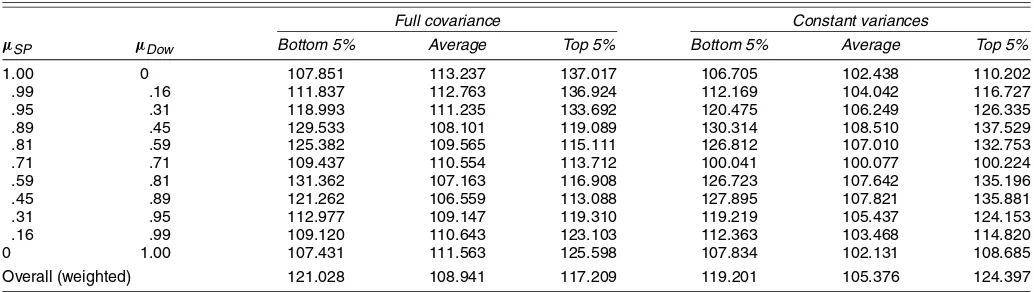
Table 11. The Importance of Extreme Correlations (S&P500 and Dow)
Full covariance Constant variances
µSP µDow Bottom 5% Average Top 5% Bottom 5% Average Top 5%
1.00 0 107.851 113.237 137.017 106.705 102.438 110.202
.99 .16 111.837 112.763 136.924 112.169 104.042 116.727
.95 .31 118.993 111.235 133.692 120.475 106.249 126.335
.89 .45 129.533 108.101 119.089 130.314 108.510 137.529
.81 .59 125.382 109.565 115.111 126.812 107.010 132.753
.71 .71 109.437 110.554 113.712 100.041 100.077 100.224
.59 .81 131.362 107.163 116.908 126.723 107.642 135.196
.45 .89 121.262 106.559 113.088 127.895 107.821 135.881
.31 .95 112.977 109.147 119.310 119.219 105.437 124.153
.16 .99 109.120 110.643 123.103 112.363 103.468 114.820
0 1.00 107.431 111.563 125.598 107.834 102.131 108.685
Overall (weighted) 121.028 108.941 117.209 119.201 105.376 124.397
NOTE: The results reported under “Full covariance” are obtained from simulations of the full covariance matrix using the Asy-DCC estimated parameters of the bivariate SP-Dow distribution. “Constant variances” means that only the dynamic correlations were simulated, while variances were kept constant at their unconditional value. The “Bottom 5%” and “Top 5%” refer to the percentiles of the distribution of conditional correlation. The numbers reported are the extra return that an investor using Asy-DCC could have required compared with an investor using constant unconditional estimators, when correlation takes on extreme values.
Table 12. Small-Sample Monte Carlo for Simulated Stocks and Bonds
T Scalar GARCH Diagonal BEKK DCC–MR Asy-DCC Constant
Full covariance
500 Scalar GARCH 19 0 0 67
Diagonal BEKK 34 1 0 60
DCC–MR 35 29 0 75
Asy-DCC 76 62 23 85
Constant 0 11 1 0
101.853 102.886 100.740 100.000 106.545
1,000 Scalar GARCH 18 0 0 93
Diagonal BEKK 58 1 0 83
DCC–MR 49 32 0 98
Asy-DCC 94 76 24 100
Constant 0 7 0 0
101.548 102.862 100.657 100.000 108.903
5,000 Scalar GARCH 24 0 0 100
Diagonal BEKK 72 0 0 80
DCC–MR 86 52 0 100
Asy-DCC 100 100 88 100
Constant 0 14 0 0
101.135 103.018 100.557 100.000 113.817
Constant variances
500 Scalar GARCH 1 3 0 15
Diagonal BEKK 18 5 4 17
DCC–MR 35 7 3 34
Asy-DCC 53 19 1 72
Constant 3 1 3 5
100.974 100.522 100.245 100.000 102.460
1,000 Scalar GARCH 0 0 0 29
Diagonal BEKK 18 1 0 35
DCC–MR 61 21 6 63
Asy-DCC 79 27 2 97
Constant 0 0 0 0
100.970 100.714 100.058 100.000 103.545
5,000 Scalar GARCH 0 0 0 90
Diagonal BEKK 38 0 0 100
DCC–MR 96 90 0 96
Asy-DCC 100 98 8 100
Constant 0 0 0 0
100.758 100.439 100.123 100.000 104.751
NOTE: The series were simulated assuming an Asy-DCC distribution with parameters estimated from the S&P500–Dow joint distribution. The top panel assumes that the whole covariance matrix is time-varying, whereas in the bottom panel variances are held constant. The number of simulations increases from 500 to 5,000. The numbers reported in the tables represent the number of times (out of 100 Monte Carlo trials) that the estimator in the row produced a significantly smaller sample variance than the model in the column. The joint Diebold and Mariano test was used to run the comparison between each pair of models. The last line of each panel reports the comparison of average (weighting expected returns according to the priors) volatilities for each method.
The Diebold–Mariano joint test confirms that there exists a group of three estimators (BEKK with variance targeting, DCC–MR, and Asy-DCC that are usually able to achieve the target of minimizing portfolio variance. When the test is re-peated for the expected returns that are closer to the true uncon-ditional mean of the assets at hand, there appears to be some significance in favor of Asy-DCC, at least in the stocks and bonds portfolio.
Simulations were used to stress the importance of having the correct time-varying information as opposed to the constant correlation often used in practice. In particular, having the cor-rect estimate of conditional correlation on those days in which this is expected to be very high or very low can be as important as 30–40% of the required return. This appears to be particu-larly true for those assets that are on average highly positively correlated.
Several more advanced questions remain to be answered by future research. The myopic portfolio allocation implemented in this article is a restriction that may somehow offset the ben-efits of having the correct covariance information at the right time. The introduction of a multistep objective function should
increase the magnitude of the values reported in this article. On the other hand, short sale constraints, which were not consid-ered in this work, should work in the opposite direction, due to the impossibility of taking extremely long or short positions when the forecasted covariance matrix would require one to do so. Given the results of the 34 assets experiment, it would be helpful if future research will investigate in greater detail the properties of DCC models in large systems.
ACKNOWLEDGMENTS
The authors thank the associate editor and two anonymous referees and seminar participants at the QFE Seminar at NYU, the European Finance Association, London Business School, and Erasmus University for helpful comments.
APPENDIX: MODELS OF CONDITIONAL COVARIANCE
In this article we use several alternative models to estimate the conditional covariance matrix. Here we provide details for the bivariate models used in the empirical analysis.