ESTIMATION OF REGIONAL FOREST ABOVEGROUND BIOMASS COMBINING
ICESAT-GLAS WAVEFORMS AND HJ-1A/HSI HYPERSPECTRAL IMAGERIES
Yanqiu Xing*, Sai Qiu, Jianhua Ding, Jing Tian
Research Centre for Forest Operations and Environment, Northeast Forestry University, Harbin 150040, P.R.China [email protected], [email protected], [email protected], [email protected]
Commission VII, WG VII/6
KEY WORDS: LiDAR, ICESat-GLAS, Waveform, HJ-1A/HSI, Hyperspectral imagery, Forest aboveground biomass, Support vector machines
ABSTRACT:
Estimation of forest aboveground biomass (AGB) is a critical challenge for understanding the global carbon cycle because it dominates the dynamics of the terrestrial carbon cycle. Light Detection and Ranging (LiDAR) system has a unique capability for estimating accurately forest canopy height, which has a direct relationship and can provide better understanding to the forest AGB. The Geoscience Laser Altimeter System (GLAS) onboard the Ice, Cloud, and land Elevation Satellite (ICESat) is the first polar-orbiting LiDAR instrument for global observations of Earth, and it has been widely used for extracting forest AGB with footprints of nominally 70m in diameter on the earth’s surface. However, the GLAS footprints are discrete geographically, and thus it has been restricted to produce the regional full coverage of forest AGB. To overcome the limit of discontinuity, the Hyper Spectral Imager (HSI) of HJ-1A with 115 bands was combined with GLAS waveforms to predict the regional forest AGB in the study. Corresponding with the field investigation in Wangqing of Changbai Mountain, China, the GLAS waveform metrics were derived and employed to establish the AGB model, which was used further for estimating the AGB within GLAS footprints. For HSI imagery, the Minimum Noise Fraction (MNF) method was used to decrease noise and reduce the dimensionality of spectral bands, and consequently the first three of MNF were able to offer almost 98% spectral information and qualified to regress with the GLAS estimated AGB. Afterwards, the support vector regression (SVR) method was employed in the study to establish the relationship between GLAS estimated AGB and three of HSI MNF (i.e. MNF1, MNF2 and MNF3), and accordingly the full covered regional forest AGB map was produced. The results showed that the adj.R2 and RMSE of SVR-AGB models were 0.75 and 4.68 t·hm-2 for broadleaf forests, 0.73 and 5.39 t·hm-2 for coniferous forests and 0.71 and 6.15 t·hm-2 for mixed forests respectively. The full covered regional forest AGB map of the study area had 0.62 of accuracy and 11.11 t·hm-2 of RMSE. The study demonstrated that it holds great potential to achieve the full covered regional forest AGB distribution with higher accuracy by combing LiDAR data and hyperspectral imageries.
* Yanqiu Xing: the corresponding author.
1 INTRODUCTION
Estimating and preserving the carbon stock in forests can help devise sequestration strategies and reduce greenhouse gas emissions(Zhang, 2014; Canadell, 2007; Miles, 2008). Forest aboveground biomass (AGB) has received more and more attention during the last decades due to its relevance to carbon cycle balancing and species diversity(Saatchi,2011a; Laurin, 2014; Saatchi, 2011b). Therefore, accurate calculation of Forest AGB and their distribution is of great significance to research on carbon cycles and carbon stocks(Neigh, 2013).
Light Detection and Ranging (LiDAR) has a unique capability for estimating forest structure parameters, especially forest vertical structure parameters. Airborne small-footprint LiDAR is considered the most accurate remote sensing technology for mapping forest AGB(Laurin, 2014; Zolkos, 2013), but its disadvantages such as expensive costs and complex data processing, limit its application on large-scale areas. On the other hand, space-borne LiDAR has a wide observation scope and can capture large-scale even global information without the limitation of time and weather(Asner, 2010; Drake, 2002).
The Geoscience Laser Altimeter System (GLAS) onboard the Ice, Cloud, and land Elevation satellite (ICESat) launched on 12 January 2003, a unique LiDAR instrument designed for continuous global observation of the earth(Zwally, 2002; Sun, 2008). It is able to capture full waveform data consists of the first return waveform reflected by forests and the last return waveform reflected by the ground. Therefore, we can obtain vertical distribution information such as forest height through analysing the full waveform data. The GLAS waveform has been widely used to estimate forest structure parameters and forest AGB(Rosette, 2008; Pflugmacher, 2008; Xing, 2010; Lefsky, 2005; Enßle, 2014; Sun, 2008). Although the GLAS performs well in estimating forest structure parameters, but its sparse distribution is discontinuity which limits its application on large-scale areas alone. The combination of multiple sources of data is required to map large areas of forest AGB(Sawada, 2015; Chi, 2015; Guo, 2010). In addition, GLAS waveform is sensitive to terrain slope due to its large footprint size, which causes overestimate of forest height and decreases forest AGB estimation accuracy.
In this paper, in order to overcome the two problems, ICESat-GLAS waveform metrics (W, I, TS) were combined with three MNF components of HJ-1A/HSI hyperspectral imageries to
estimate forest AGB based on Support Vector Regression (SVR) method in order to improve the forest AGB estimation accuracy and achieve the full covered regional forest AGB distribution.
2 MATERIALS
2.1 Study area
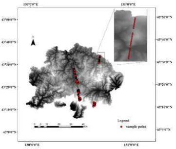
The study area is within Wangqing forestry of Jilin province, China, and is located along the border between China and North Korea (43°05′N-43°40′N, 129°56′E-131°04′E) (see Figure 1). It belongs to Changbai mountain system, one of the most valuable reserves in China, and it is a rich gene pool of many plant species. The elevation ranges from 360m to 1477m, and the terrain slope generally ranges from 0° to 45°. The study area is dominated by cool temperate continental climate with four clearly defined seasons. The dominant species are Korean pine (Pinus koraiensis Siebold & Zucc.), Spruce (Picea
Figure 1. Study area and the location of sample points
2.2 ICESat-GLAS waveform
ICESat-GLAS carries three lasers in total, and each laser emits 40 pulses of 1064 nm per second, resulting in an elliptical footprint of ~70m diameter on the surface of the earth, with each footprint separated by 172m(Schutz, 2005). GLAS totally offers fifteen kinds of products(Sun, 2008). In the study, release-31 of the GLA01 and GLA14 data were acquired through the National Snow and Ice Data Center (NSIDC) web-site (http://nsidc.org/data/icesat/). The GLA01 data contains raw waveform data. For land surfaces, the waveform has 544 bins with one bin represents 15cm. The GLA14 data does not contain waveform data, but includes information about the observation conditions and the latitude and longitude of footprints, etc. The two products are joined together by the record index of the GLAS footprints.
Since GLAS waveforms was easily affected by clouds and system noise, cloud-contaminated and abnormal waveforms were removed before extracting waveform parameters by using the saturation-free flag (i_satNdx=0) and cloud-free flag (i_FRir_qaFlg=15) data extracted from GLA14 product(Popescu, 2011).
2.3 HJ-1A HSI imageries
The Disaster and Environment Monitoring and Forecast constellation consists of two satellites (HJ-1A and HJ-1B), and was launched on September 6, 2008. HJ-1A is equipped with a Hyper Spectral Imager (HSI) with 50km swath and 100 m spatial resolution consisting of 115 bands with 4.32nm spectral resolution in the 0.45~ 0.95μm range. Four images of level-2 data were acquired through the China Centre for Resources Satellite Data and Application web site and used for Forest AGB estimation (http://www.cresda.com/n16/index.html).
2.4 Field inventory data
The field data collection was carried out in September of 2006 and 2007 in the study area and 183 circular plots of 500 m2 along ICESat-GLAS flight track direction were randomly established. The description of field data was listed in Table 1. These plots consist of 101 broad-leaved forest, 38 coniferous forest and 44 mixed forest. In each plot, we recorded species and forest canopy density. Tree height and DBH (Diameter at Breast Height) were also measured with a DBH greater than 10 cm. For trees with a DBH between 4cm and 10cm, we only 2008). In the study, the sum of the single tree biomass divided by plot area was defined as the forest aboveground biomass of each plot.
biomass/t·hm-2 112.41 15.78 63.64
Table.1 Description of field data
3 METHOD
3.1 Data processing
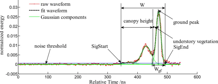
3.1.1 ICESat-GLAS waveform processing and metrics extraction: The GLAS waveforms were smoothed by Gaussian filter to remove noise. The smoothed waveform was modelled with Gaussian components using the algorithm developed by Brenner et al(Brenner, 2003). The signal start and signal end were identified using the background noise threshold which was set to the mean background noise plus 4.5 times the background noise standard deviation(Lefsky, 2005).
Generally, waveform extent (W) as shown in Figure 2 was defined as maximum forest height on a flat area. But the waveform was increased as the function of terrain slope and footprint size in mountain forests. To increase the accuracy of maximum forest height and forest AGB, the terrain slope parameter TS was extracted from the GLAS waveform based on an approach developed by Mahoney(Mahoney, 2014) in order to reduce the associated uncertainties, The equations are shown in Equation (1).
Where TS =terrain slope
In this paper the forest canopy density was calculated for each footprint as the ratio of the forest canopy energy to the total waveform from signal start to signal end.
I E E
v/
(2)Figure 2. The GLAS waveform and GLAS parameters
3.1.2 HJ-1A/HSI imageries processing and metrics extraction: The atmospheric corrections for the four images were performed using the FLAASH (Fast line-of-Sight Atmospheric Analysis of Spectral Hypercubus) algorithm, which is based on the MODTRAN4+ Radiative transfer model. The study area was classified into broadleaf forest, coniferous forest, mixed forest and non-forest areas by the supervised classification method with the help of forest inventory data. Because HSI hyperspectral image consists of 115 bands, there is strong data redundancy and high correlation between neighboring bands. In the study, the Minimum Noise Fraction (MNF) method was applied to decrease noise and reduce the dimensionality of spectral bands. The first three MNF components (i.e. MNF1, MNF2 and MNF3) contains almost 98% of total information and satisfies research requirement and so they were used to do forest AGB estimation. Considering that the spatial resolution of GLAS data and HSI data are different, circle buffers of 70m in diameter were established on the HSI image with the coordinate of GLAS footprints as their center, and the mean value of pixels covered by circle buffers was defined as MNF value of the corresponding GLAS footprints.
3.2 Regional forest AGB estimation combining GLAS waveform and HJ-1A/HSI imageries
In the study, GLAS waveform and HSI image were combined to estimate forest AGB. Metrics (W, TS, I) derived from GLAS data and field AGB were used to develop the GLAS-AGB models by multiple regression method for different forest types in the study area. The GLAS-AGB models were then used to calculate forest AGB of the remaining GLAS footprints.
The SVR (Support Vector Regression) method was applied to combine the GLAS metrics with HSI metrics to finish regional forest AGB estimation. SVR is based on statistical learning theory and the structural risk minimization principle. It performs well in approximating and generalizing. The basic principle of SVR is to map the data into a high dimensional feature space via a kernel function, after which a linear regression is performed in this feature space. The radial basis function is a normal kernel function as shown in Equation(3):
( , ) exp(
2)
estimation. To build the SVR-AGB model, all the forest AGB of GLAS footprints and the correlated three MNF components of HSI data were put into LIBSVM, and they were randomly divided into training and validation data to develop SVR-AGB models for three forest types. The SVR-AGB models were then used to calculate forest AGB of each pixel of HSI data and the AGB map of the entire study area was achieved. The flow chart of the forest AGB map process is shown in Figure 3.The adjusted coefficient of determination (adj.R2) was used to evaluate the goodness of fit for the model. The root mean square error (RMSE) was used to assess the error between the estimated AGB and field-observed AGB at the footprint level.
Field inventory
data
Biomass of forest stands
GLAS waveforms
HJ-1A/HSI hyperspectral
data
Biomass of plots
Pre-processing
Waveform parameters extration
Biomass GLAS model Biomass SVR model
Biomass map
Forest classification MNF
Figure 3. Flow chart of regional biomass estimation from GLAS, HJ-1A/HSI, and field data
4 RESULTS AND DISCUSSION
4.1 Biomass estimation from GLAS waveform parameters
As shown in Figure 4, TS has a strong linear relationship with terrain slope (adj.R2=0.78, RMSE=4.74°). Therefore, TS can be used to correct the influence of terrain slope on GLAS waveform for further forest AGB estimation.
As shown in table 2, when the under-story vegetation height was set as 2m, the accuracy was the highest (adj.R2=0.64, RMSE=0.13). Thus in this study, the GLAS parameter I extracted from the GLAS waveform when the under-story
vegetation height was set as 2m was used to estimate forest AGB.
Figure 4. Scatter plot of TS and terrain slope
Under story vegetation
height adj.R2 RMSE
1m 0.52 0.21
2m 0.64 0.13
3m 0.60 0.20
Table.2 Adj.R2 and RMSE value of GLAS forest canopy density model with different under story vegetation height
Forest type parameters adj.R2 RMSE
(t·hm-2) N
W 0.39 18.64
W,TS 0.45 16.23
W,I 0.53 11.92
Broadleaf forest
W,TS,I 0.65 10.21
68
W 0.36 20.25
W,TS 0.53 16.61
W,I 0.59 11.92
Coniferous forest
W,TS,I 0.66 11.86
25
W 0.46 19.56
W,TS 0.52 15.19
W,I 0.58 13.72
Mixed forest
W,TS,I 0.62 12.85
29
Table.3 Results of AGB estimation models with GLAS parameters
Validation results
Forest types Equation adj.R2 RMSE
(t·hm-2) Broadleaf forest
B
0.87
W
0.09
D
tan( ) 56.95
TS
I
0.75
0.75 8.72 Coniferous forestB
0.65
W
0.12
D
tan( ) 55.41
TS
I
7.36
0.77 8.38 Mixed forestB
1.17
W
0.14
D
tan( ) 49.73
TS
I
5.23
0.76 7.60Table.4 Regression equations of AGB models of the three forest types
As shown in Table 3, when W and TS were considered in the regression analysis, adj.R2 significantly increased and RMSE significantly declined. For example, adj.R2 increased from 0.39 to 0.45 in broadleaf forests, from 0.36 to 0.53 in coniferous forests and from 0.46 to 0.52 in mixed forests. RMSE declined from 18.64 t·hm-2 to 16.23 t·hm-2 in broadleaf forests, from 20.25 t·hm-2 to 16.61 t·hm-2 in coniferous forests, and from 19.56 t·hm-2 to 15.19 t·hm-2 in mixed forests, respectively. Additionally, from the Table 3, it can also be seen that the adj.R2 value of AGB models with W and I as independent variables of the three forest types significantly increased, demonstrating that forest AGB really has linear relationship with I. When all of the GLAS parameters (W, TS, I) were considered in the AGB models, the accuracy was the best. In this case, adj.R2 and RMSE values of the forest AGB model are 0.65 and 10.21 t·hm-2 for broadleaf forests, 0.66 and 11.86 waveforms and the forest AGB calculated from forest inventory data has good consistency with adj.R2=0.75 for broadleaf forest, adj.R2=0.77 for coniferous forest and adj.R2=0.76 for mixed forest. Therefore, GLAS-AGB estimation models can be used to predict regional forest aboveground biomass combining with HJ-1A/HSI data in further study.
4.2 Regional AGB estimates and validation
The regional SVR-AGB models are shown in Table 5. It can be seen that the accuracy of broadleaf forest was higher than coniferous forest and mixed forest. The forest AGB of the study area was calculated using the SVR-AGB model pixel-by-pixel. The final results are shown in Figure 5, and it could be seen that the forest AGB of the study area ranges from 0 to 164 t·hm-2. The highest forest AGB is located in the northern and southwestern part of the study area where evergreen trees are dominant. The southern and northeastern parts of the study area are dominant with larch whose leaves had become yellow or fallen, resulting in a lower AGB value. The regions of the study area with a forest AGB value of zero are mainly residential areas, roads and rivers.
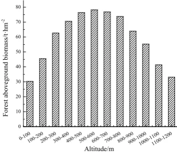
Even though the accuracy of forest AGB estimation was improved, there is also some bias between the predicted forest AGB and field forest AGB, and the reasons are various. As shown in Figure 5, the forest AGB increases as altitude increases and then declined when the altitude reached 700m. Large amounts of forest AGB were concentrated in the altitudes between 400m and 800m. Because the study area is dominated by a cool temperate continental climate, when the altitude reached 1000m, the temperature is only 3 , which is not ℃
suitable for plants, and there were only some small but old trees. The time of acquisition of the data in the study was different, which may also bring some negative influence on the results.
Training result Testing result
Forest type parameters adj.R2 RMSE
(t·hm-2) adj.R2 (t·hmRMSE -2)
Broadleaf forest MNF1,MNF2,MNF3 0.75 4.68 0.70 6.32
Coniferous forest MNF1,MNF2,MNF3 0.73 5.39 0.67 10.25
Mixed forest MNF1,MNF2,MNF3 0.71 6.15 0.63 12.34
Table.5 Results of forest AGB models estimated with HJ-1A/HSI parameters
developed through combining ICESat-GLAS and HJ-1A/HSI.
The results demonstrated that GLAS waveform plays an important role in linking field inventory data to HJ-1A/HSI data, because of the fact that the acquisition of field inventory data is both time-and resource consuming. GLAS waveform
records the interaction of laser beams with forest and ground which reflect the vertical structure of forest. Some GLAS parameters such as W, I, and TS can be used to develop a forest AGB model. TS has a strong relationship with terrain slope, and can be used to correct the influence of terrain slope on the GLAS waveform. The ratio I of the forest canopy energy to the total energy of GLAS waveform has the best correlation with forest canopy density when the under-story vegetation height was 2m. And the results showed that GLAS waveform parameters have the good relationship with AGB and the AGB equations for the three forest types can be used to obtain sample biomass data for regional AGB estimation using HJ-1A/HSI images.
GLAS parameters which reflecting forest vertical and horizontal structure are considered in the AGB model, and the accuracy of forest AGB model is improved, comparing with that alone using vertical structure or horizontal structure parameters.
From the results shown in Table 5, we can see that the combination of GLAS data and HJ-1A/HSI data is reasonable and promising for regional forest AGB estimation. Combining GLAS and HJ-1A/HSI data can improve the estimation accuracy of forest AGB and can complete regional forest AGB estimation. However, because of the spatial resolution of HJ-1A/HSI data, the spatial distribution and the limitation number of GLAS footprints, the accuracy of the estimated forest AGB of the study area was not very high. In the future studies, some high spatial resolution and high spectral resolution image data can be considered to improve the accuracy.
REFERENCES
Asner G.P., 2010. High-resolution forest Carbon stocks and emissions in the Amazon. Proceedings of the National Academy of Sciences, 107(38): 11674-16738.
Brenner A.C., 2003. Derivation of range and range distributions from laser pulse waveform analysis for surface elevations, roughness, slope, and vegetation heights. Algorithm Theoretical Basis Document, 4: 26-32.
Canadell J.G., 2007. Contributions to accelerating atmospheric CO2 growth from economic activity, Carbon intensity, and efficiency of natural sinks. Proceedings of the National Academy of Sciences, 104(47): 11887-18866.
Chi H., 2015. National forest aboveground biomass mapping from ICESat/GLAS data and modis imagery in China. Remote Sensing, 7(5): 5534-5564.
Deo R.K.. 2008. Modelling and mapping of aboveground biomass and Carbon sequestration in the cool temperate forest of North-east China. Netherlands: International Institiute For Geo-information Science and earth observation enschede.
Drake J.B., 2002. Sensitivity of large-footprint lidar to canopy structure and biomass in a neotropical rainforest. Remote Sensing of Environment, 81(2): 378-392.
Enßle F., 2014. Accuracy of vegetation height and terrain elevation derived from ICESat/GLAS in forested areas. International Journal of Applied Earth Observation, 31: 37-44.
Guo Z., 2010. Estimating forest aboveground biomass using
HJ-1 Satellite CCD and ICESat GLAS waveform data. Science China Earth Sciences, 53(1): 16-25.
Laurin G.V., 2014. Above ground biomass estimation in an African tropical forest with lidar and hyperspectral data. Isprs Journal of Photogrammetry and Remote Sensing, 89: 49-58.
Lefsky M.A., 2005. Estimates of forest canopy height and aboveground biomass using ICESat. Geophysical Research Letters, 32(22).
Mahoney C., 2014. Slope estimation from ICESat/GLAS. Remote Sensing, 6(10): 10051-11006.
Miles L., 2008. Reducing greenhouse gas emissions from deforestation and forest degradation: global land-use implications. Science, 320(5882): 1454-1455.
Neigh C.S., 2013. Taking stock of circumboreal forest Carbon with ground measurements, airborne and spaceborne LiDAR. Remote Sensing of Environment, 137: 274-287.
Pflugmacher D., 2008. Regional applicability of forest height and aboveground biomass models for the Geoscience Laser Altimeter System. Forest Science, 54(6): 647-657.
Popescu S.C., 2011. Satellite lidar vs. small footprint airborne lidar: Comparing the accuracy of aboveground biomass estimates and forest structure metrics at footprint level. Remote Sensing of Environment, 115(11): 2786-2797.
Rosette J., 2008. Vegetation height estimates for a mixed temperate forest using satellite laser altimetry. International Journal of Remote Sensing, 29(5): 1475-1493.
Saatchi S.S., 2011A. Benchmark map of forest Carbon stocks in tropical regions across three continents. Proceedings of the National Academy of Sciences, 108(24): 9899-9904.
Saatchi S., 2011B. Impact of spatial variability of tropical forest structure on radar estimation of aboveground biomass. Remote Sensing of Environment, 115(11): 2836-2849.
Sawada Y., 2015. A new 500-m resolution map of canopy height for Amazon forest using spaceborne LiDAR and cloud-free MODIS imagery. International Journal of Applied Earth Observation, 43: 92-101. International Journal of Applied Earth Observation, 12(5): 385-392.
Zhang G., 2014. Estimation of forest aboveground biomass in California using canopy height and leaf area index estimated from satellite data. Remote Sensing of Environment, 151: 44-56.
Zolkos S.G., 2013. A meta-analysis of terrestrial aboveground
biomass estimation using lidar remote sensing. Remote Sensing
of Environment, 128: 289-298. Zwally H.J., 2002. ICESat's laser measurements of polar ice, atmosphere, ocean, and land. Journal of Geodynamics, 34(3): 405-445.