ANALYSIS OF LANDSLIDES BASED ON DISPLACEMENTS OF LINES
A. T. Mozas-Calvache a *, J. L. Pérez-García a, T. Fernández-del Castillo a, J. M. Gómez-López a, C. Colomo-Jiménez a
a
Dept. Ingeniería Cartográfica, Geodésica y Fotogrametría, University of Jaén, 23071 Jaén, Spain (antmozas, jlperez, tfernan, jglopez, ccolomo)@ujaen.es
Commission VII, WG VII/5
KEY WORDS: UAS, photogrammetry, landslide, road, linear elements
ABSTRACT:
Nowadays, the development of UAS has allowed the obtaining of high resolution and accurate cartographic products, such as DSMs and orthoimages. These products can be used in studies of the evolution of landslides. The stability of slopes is a main issue because, among others, it can suppose a serious risk to infrastructures. Until this moment, some studies for analysing slope movements have been carried out using the comparison of positions of well-defined points or comparing two surfaces obtained from two DSMs. In this paper we present a methodology for analysing landslides based on some linear elements located on the terrain. More specifically, we analyse some lines of road sections which are located on an unstable slope, checking the movements of the landslide and their effect on the infrastructure. The methodology includes the obtaining of high resolution orthoimages and DSMs which correspond to two or more epochs of the same landslide, the 3D digitizing of common linear elements, and the computing of the displacements of matched lines (from two epochs) using positional control methods based on lines. The proposed methodology has been tested using two DSMs and two orthoimages (corresponding to two epochs) obtained from two photogrammetric projects developed with an UAS. This real case was applied to an unstable slope with landslides which affected several sections of a road. The results have demonstrated the viability of the proposed methodology in analysing the behaviour of the landslide and more specifically, the effects on these infrastructures.
1. INTRODUCTION
The analysis of landslides, including their temporal evolution, is an important issue to be considered because of their potential hazards for people, infrastructures, etc. Knowledge of the behaviour of landslides can allow the prevention of damage (e. g. to infrastructure), anticipating the effects by means of the application of corrective measures. A landslide is defined in a simple way as "the movement of a mass of rock, debris, or earth down a slope" (Cruden, 1991).
Until this moment, some studies for analysing slope movements have been carried out using the comparison of positions of well-defined points or by comparing two surfaces obtained from two Digital Surface Models (DSMs). In this context, several techniques have been developed for this goal and applied with success. Firstly, the acquisition techniques based on the measure of discrete points of the terrain, such as total stations (Tsai et al., 2012) or Global Positioning Systems (GPS) (Gili et al., 2000), or more generally Global Navigation Satellite Systems (GNSS). A more continuous sample of points is achieved when using Terrestrial Laser Scanning (TLS). In this case, the number of points acquired can be more than several million. So TLS allows DSMs to be obtained with the appropriate resolution to be used for analysing landslide movements (Abellán et al., 2006; Travelletti et al., 2008; Monserrat and Crosseto, 2008). However, the main issue associated with these terrestrial techniques is that related to accessibility and visibility. A further step is given by photogrammetric and remote sensing techniques (Metternich et al., 2005; Fernández et al., 2009; Scaioni et al., 2014) and LiDAR (Jaboyedoff et al., 2012). From traditional aerial photogrammetry (Brunsden and Chandler, 1996; Walstra et al., 2004; Prokešová, et al., 2010) to the current development of
Unmanned Aircraft Systems (UAS) (Stumpf et al., 2012; Niethammer et al., 2012; Turner et al., 2015; Fernández et al., 2015), the use of photogrammetric flights, many times combined with LiDAR data (Dewitte et al., 2008; Corsini et al., 2009; Fernández et al., 2012), for modelling landslides has suffered an enormous increment because of the high geometric accuracy achieved, the semantic information of images, the easy accessibility in the field and the reduction of costs in the case of UAS. Furthermore, the photogrammetric techniques allow a DSM of the terrain to be obtained and also orthoimages. These cartographic products can help us understand the behaviour of the landslide. Obviously, the selection of the technique will be related to the number of points to be acquired and the accuracy of the system. The requirements of accuracy are mainly related to the range of displacements to be detected. In this sense, Nex and Remondino (2014) showed a graph where the use of the geomatic techniques is delimited depending on the zone dimensions and complexity (number of points), and Siebert and Teizer (2014) provided a comparison between the required accuracy and the area of the zone of study. A more detailed description of landslide instrumentation and monitoring techniques is shown in Margottini et al. (2013).
promising tool for landslide recognition (Scaioni et al., 2014). In this context there are several studies that have used photogrammetric products obtained from UAS flights in order to study and analyse landslides, as in natural slopes (Niethammer et al., 2012; Turner et al., 2015; Fernández et al., 2015) such as road embankments (Carvajal et al., 2011). These studies have mainly analysed DSMs or discrete points extracted from landslides at a determined moment or comparing them between several epochs. The first and simplest approach used by several authors has been the comparison of DSMs corresponding to several epochs (Stumpf et al., 2012; Niethammer et al., 2012; Turner et al., 2015; Fernández et al., 2015) in order to analyse the evolution of a landslide. In other cases, DSM have been used to identify point features automatically; in this sense, a common issue of these studies is the use of points (extracted from DSMs or orthoimages), in a manual (Fernandez et al., 2015) or automatic way (Lucieer et al., 2014; Turner et al., 2015) for modelling the displacements. Nevertheless, there is the possibility of analysing lines instead of points due to the usual presence of some linear elements in landslides (e. g. roads, fissures, etc.). Stumpf, et al., (2012), Niethammer et al. (2012) and Akcay (2015) analysed the landslide fissures obtained from DSMs and applied textural filters to identify active zones in the landslides, but until now lines have not been used to measure displacements. In this way, the analysis of the displacements of several epochs could give a complete model of the behaviour of the landslide if the lines are well-distributed and also the effects of the movements on some infrastructures involved in the landslide. Furthermore, the analysis of lines could allow the behaviour of these elements to be studied jointly (e.g. as a rigid block) in contrast with the discrete study of points. In any case, the displacements between epochs of some digitized lines from photogrammetric UAS projects can be determined, and a model of the behaviour of these elements can be derived from these values. This is the main hypothesis of this study.
The analysis of the displacements of linear elements has not been studied until this moment in this context. However, in the positional control of cartographic products there are some studies which have controlled a sample of lines. Several methodologies have been described for determining the positional accuracy of lines, starting from the initial concept of the uncertainty band of a line (given by Perkal, 1956), to the current models (Shi and Liu, 2000). In addition, some positional control methods have also been described derived from these models (Mozas and Ariza, 2010). The main positional control methodologies based on lines, described until this moment, are based on the determination of uncertainty using distance calculations (Skidmore and Turner, 1992; Abbas et al., 1995; Mozas and Ariza, 2011 and Mozas and Ariza, 2015) or buffer determination (Goodchild and Hunter, 1997). These methodologies can be used or adapted for modelling the displacements of linear elements involved in a landslide.
To summarize, in this paper we present a methodology for analysing landslides based on some linear elements located on the terrain. More specifically, we analyse some lines digitized from some road sections which are located on an unstable slope. In this way we can analyse both the movements of the slope and their effects on the infrastructure. This analysis could detect the possible existence of specific movements of the infrastructure caused by its particular behaviour (e. g. a drainage structure can act as a rigid block). The proposed methodology has been checked using two orthoimages of 5 centimetres of spatial resolution and two DSMs, obtained from two photogrammetric
studies. The photographs were obtained from a UAS flight over an unstable slope with landslides which affected several sections of a road. This application has been carried out during two epochs (with four months of difference). The results have demonstrated the viability of the proposed methodology in analysing the behaviour of these infrastructures and the landslides.
2. METHODOLOGY
The methodology proposed in this study is summarized in Figure 1.
Figure 1. Proposed methodology
Firstly, a common process for developing two UAS photogrammetric flights is carried out during two epochs. This process includes the planning of the flight (repeated in both epochs), the orientation of the photographs, the obtaining of the Digital Surface Model (DSM) and subsequently, the obtaining of an orthoimage, according the methodology followed in previous works (Fernández et al., 2015). The DSMs and the orthoimages of both epochs are the final products derived from the photogrammetric process used in this study.
linear elements are obtained (one from each epoch). Both sets of lines are composed of the same quantity of lines and vertexes.
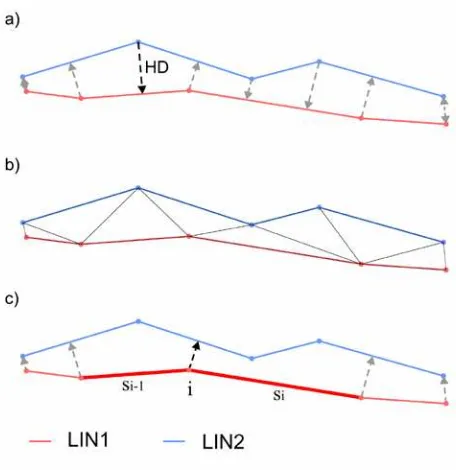
Figure 2. Methods based on lines used in this study
Thirdly, the main step of this methodology is related to the control of lines. The two sets of lines are compared using three different methods based on lines both in 2D and 3D in order to analyse the behaviour of height component. The first control method is related to the determination of the Hausdorff Distance (HD) (Abbas et al., 1995) between the homologous lines. The calculation consists of the determination of the maximum distance between the vertexes of the line of LIN1 and the line of LIN2 (Figure 2a) and vice versa. This method provides an estimation of the maximum displacement between the lines. The second is called Mean Displacement (MD). This method was originally described by Skidmore and Turner (1992) for 2D lines and was extended to 3D lines by Mozas and Ariza (2015). It consists of the determination of the enclosed area between both homologous lines divided by the length of the line. The determination of the enclosed area for 3D lines was solved by Mozas and Ariza (2015) using a 3D triangulation between the lines (Figure 2b). The third method to be applied is the VIM method (Mozas and Ariza, 2011), which provides values of mean displacement (VIM-D) and average increments (VIM-I). This method consists of the calculation of the Euclidean distances and the increments of coordinates from the vertexes of the control line (for example, i in Figure 2c) to the line to be controlled and the weighting of these values by the length of the adjacent segments to the implicated vertex (si-1 and si in Figure 2c). The final results are a mean value of displacement and three mean values of increments (X, Y and Z). In this case, the lines of the first epoch (LIN1) are considered as control lines and LIN2 are selected as those to be controlled (following the notation given by Mozas and Ariza, 2011). The final stage of the methodology is that related to the analysis of the results obtained in the previous step.
3. APPLICATION
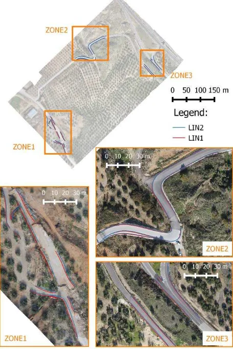
This methodology is applied to the real case of an unstable slope close to the A-44 highway in Jaén (Spain) (Figure 3). In
this zone there are several active landslides (Fernández et al., 2015). In this case we analysed two active sections (Figure 3) or landslides which correspond to mud flows, according to the classification of Varnes (1978). Following the proposed methodology two UAS photogrammetric projects (called UAS1 and UAS2) were developed with a temporal interval of about 4 months (November of 2012 and March of 2013). These epochs correspond to dry and wet seasons in this location.
Figure 3. Zone of study and landslides.
set of lines called LIN1. The planimetric digitizing was carried out using QGISTM software. After that, ArcGISTM software was used for determining the height of each vertex (using the DSM1 as reference). The LIN1 was copied (LIN2) and the vertexes of the lines were moved to the new positions that appeared in ORTHO2. Finally, the process of obtaining height values was repeated on LIN2, using DSM2 in this case.
Figure 4. Datasets LIN1 and LIN2 of digitized lines over ORTHO1. Division by zones.
Thus the final dataset was composed of 23 lines defined by 390 vertexes and a total length of about 1000 metres (Figure 4). We divided the zone of study into 3 sectors considering 3 separate zones where the lines were affected by the landslides. These 3 sectors were called ZONE1 (Figure 4a), ZONE2 (Figure 4b) and ZONE3 (Figure 4c). The zones were selected and located inside the unstable slope in order to analyse the behaviour of the landslides. ZONE1 was located at the head of the main landslide, according to IAEG (1990) terminology. ZONE 2 was in an intermediate zone which was affected by a secondary landslide separate from the main one. This landslide was situated on the northern flank of the unstable slope. Finally, ZONE3 was located at the foot of the main landslide close to the highway (IAEG, 1990).
The final step consisted of the application of positional control based on lines to both datasets of lines both in 2D and 3D cases. This stage was implemented using a specific application developed in JAVATM for this purpose.
4. RESULTS AND DISCUSSION
A summary of the 3D lengths of the lines LIN1 and LIN2 is shown in Table 1. The general behaviour is an increase of the length of the lines of about 0.4%. The analysis by zones shows this increase in ZONE1 and ZONE2. However, ZONE3 shows little reduction of its length.
Total ZONE1 ZONE2 ZONE3
metres metres metres metres LIN1 976.067 323.925 413.584 238.559 LIN2 980.124 326.643 415.054 238.427
Variation 0.4% 0.8% 0.4% -0.1%
Table 1. 3D Lengths of LIN1 and LIN2
The results of the application of the control methods to LIN1 and LIN2 are presented divided by method, by case (2D and 3D) and by zone in Table 2. The results of the HD method show mean displacement values of about 1 metre (2D and 3D), with a difference between 2D and 3D of about 13 centimetres. The analysis by zone shows higher values in ZONE1 (both 2D and 3D) with respect to the others. This indicates the existence of some singular displacements in this head zone of the landslide.
Metric Total ZONE1 ZONE2 ZONE3
metres metres metres metres
HD 2D 0.993 1.855 0.531 0.620
HD 3D 1.124 1.972 0.698 0.712
MD 2D 0.638 1.227 0.274 0.468
MD 3D 0.708 1.326 0.337 0.514
VIM-D 2D 0.649 1.239 0.289 0.468
VIM-D 3D 0.708 1.329 0.335 0.514
VIM-I X 0.432 0.969 0.056 0.354
VIM-I Y 0.375 0.614 0.230 0.303
VIM-I Z 0.026 -0.149 0.095 0.146
Table 2. Mean results of HD, MD and VIM
In the case of the MD method, the mean values of displacements are close to 0.64 metres in 2D. We have to note that the influence of height is not too great because the increase of the value of displacement when including this component is only 7 centimetres. The results by zone are consistent with those shown for the HD method. ZONE1 shows higher values of displacement (more than 1.2 metres in 2D and 1.3 metres in 3D), but in the other zones the values are lower. The lowest values of displacement are found in ZONE2.
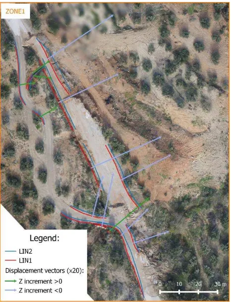
Figure 5. Displacement vectors (20x) from VIM-I in ZONE1.
The mean results presented in Table 2 are confirmed with the graphical analysis of specific displacements of the lines. Figure 5, Figure 6 and Figure 7 show the displacement vector for each line obtained using VIM-I values. For an easy interpretation, the vectors are represented multiplying the modules by a 20 factor in XY and colouring the vector according to the Z increment (positive or negative). Figure 5 shows the displacement vectors of ZONE1. There are some parallel vectors in the northeastern direction (on the right) with higher values of displacement and negative values of Z increment. This zone corresponds to the area nearest to the main scarp of the landslide. More to the left, the vectors show more variability with positive and negative values of Z increments.
Figure 6 shows the displacement vectors of ZONE2. In this case the vectors show similar behaviour with parallel directions closer to North than the previous case. This is coherent because this landslide is isolated from the other and its direction is slightly different. All vectors show positive Z increments. Finally, Figure 7 shows the displacements obtained in ZONE3. In this case, the vectors also show similar directions with respect to those of ZONE1 (to the northeast) and the Z increments are positive in all cases.
The results have shown the evolution of the lines analysed between both epochs and as a consequence the behaviour of the landslides. In general, the displacement in XY shows values of 0.6-0.7 metres with directions approximated to the northeast. The Z component shows more variability because there are some negative increments in ZONE1 (the nearest parts to the main scarp). Thus the general behaviour suggests a transfer of material in the northeast direction which is accumulated, and as consequence there is an elevation of the terrain and more specifically of the infrastructures analysed. The differences of
direction found in the vectors of ZONE2 are also coherent if we consider that this zone is isolated from the main landslide.
Figure 6. Displacement vectors (20x) from VIM-I in ZONE2.
Figure 7. Displacement vectors (20x) from VIM-I in ZONE3.
The analysis of the variation of the length of lines by zones indicates that the lines in ZONE1 suffered greater deformations (about 2.5 metres) than the other lines. In general there are increases of length in the evolution of the lines. This is coherent with the type of landslides of this zone corresponding to flows (Fernández et al., 2015) in which mass deformations produce an expansion of the features. The lines of ZONE3 show a small reduction in length (about 10 centimetres) but this value is not significant. To summarize, the values of length, displacements and increments obtained are coherent considering the characteristics of the unstable slope and the location and particularities of each zone, and the methodology has been able to detect these movements.
5. CONCLUSIONS
analysis of lines included in the landslide allows information to be obtained about the kinematics of the landslide and also about the behaviour of the affected infrastructure (e. g. roads). The methodology includes the obtaining of two datasets of lines digitized from two UAS projects performed during two epochs. The lines are obtained from an orthoimage and a DSM in each epoch. After that, the displacements of lines are checked using some positional control procedures based on lines. We have to highlight the implementation of these procedures in 3D. This supposes an important step for this work in contrast to the traditional use of lines in 2D in positional control procedures.
The application to a real case has demonstrated the viability of the proposed methodology because it has detected the displacements of lines and as a consequence the behaviour of each landslide can be known. The displacement values obtained are reliable because they are much higher than the positional accuracy given by the acquisition technique (estimated at 5 centimetres). The analysis by zones has also shown to be very interesting because of the possibilities of finding particular behaviours in displacement directions or changes in heights.
This study has to be understood as a preliminary work. Future work will deal with advances in the methodology, adapting control procedures to this goal, the extension to other types of lines (e. g. fissures), the employment of more UAS flights, analysis of the sample size, accuracies, etc.
ACKNOWLEDGEMENTS
This work has been supported by the project ISTEGEO RNM-06862 (Andalusian Research Plan), the Advanced Studies Centre on Earth Sciences (CEACTierra) and the PAIDI Research Group TEP-213.
REFERENCES
Abbas, I., Grussenmeyer, P. and Hottier, P., 1995. Contrôle de la planimétrie d’une base de données vectorielles: une nouvelle méthode basée sur la distance de Hausdorff: la méthode du contrôle linéaire. Revue de la Société Française de Photogrammétrie et de Télédétection, 137(1), pp. 6-11.
Abellán, A., Vilaplana, J.M. and Martínez, J., 2006. Application of a long-range Terrestrial Laser Scanner to a detailed rockfall study at Vall de Núria (Eastern Pyrenees, Spain). Engineering Geology, 88(3-4), pp. 136-148.
Akcay, O., 2015. Landslide fissure inference assessment by ANFIS and logistic regression using UAS-based photogrammetry. ISPRS International Journal of Geo-Information, 4(4), pp. 2131-2158.
Brunsden, D. and Chandler, J.H., 1996. Development of an episodic landform change model based upon the Black Ven mudslide, 1946-1995. In: Anderson, M. G. and Brooks, S. M. (eds.) Advances in Hillslope Processes. John Wiley & Sons Ltd., Chichester, pp. 869-896.
Carvajal, F., Agüera, F. and Pérez, M., 2011. Surveying a landslide in a road embankment using unmanned aerial vehicle photogrammetry. International Archives of Photogrammetry, Remote Sensing and Spatial Information Sciences, Zurich, Switzerland, Vol. XXXVIII-1/C22, pp. 201–206.
Colomina, I., and Molina, P., 2014. Unmanned aerial systems for photogrammetry and remote sensing: A review. ISPRS Journal of Photogrammetry and Remote Sensing, 92, pp. 79-97.
Corsini, A., Borgatti, L., Cervi, F., Dahne, A., Ronchetti, F. and Sterzai, P., 2009. Estimating mass-wasting processes in active earth slides-earth flows with time-series of High-Resolution DEMs from photogrammetry and airborne LiDAR. Natural Hazards and Earth System Sciences, 9, pp. 433-439.
Cruden, D. M., 1991. A simple definition of a landslide. Bulletin of Engineering Geology and the Environment, 43(1), pp. 27-29.
Dewitte, O., Jasselette, J.C., Cornet, Y., Van Den Eeckhaut, M., Collignon, A., Poesen, J. and Demoulin, A., 2008. Tracking landslide displacement by multi-temporal DTMs: a combined aerial stereophotogrammetric and LiDAR approach in Belgium, Engineering Geology, 99, pp. 11-22.
Fernandez, P., Irigaray, C., Jimenez, J., El Hamdouni, R., Crosetto, M., Monserrat, O. and Chacon, J., 2009. First delimitation of areas affected by ground deformations in the Guadalfeo River Valley and Granada metropolitan area (Spain) using the DInSAR technique. Engineering Geology, 105(1), pp. 84-101.
Fernández, T., Pérez J.L., Colomo, C., Mata, E., Delgado, J., Cardenal, F.J., Irigaray, C. and Chacón, J., 2012. Digital Photogrammetry and LiDAR techniques to study the evolution of a landslide. In 8th Gi4DM (Geinformation for Disaster Management), Enschede, The Netherlands, pp. 95-104.
Fernández, T., Pérez, J. L., Cardenal, F. J., López, A., Gómez, J. M., Colomo, C., Delgado, J. and Sánchez, M., 2015. Use of a light UAV and photogrammetric techniques to study the evolution of a landslide in Jaén (southern Spain). The International Archives of Photogrammetry, Remote Sensing and Spatial Information Sciences, La Grande Motte, France, Vol. XL-3/W3, pp. 241-248.
Gili, J. A., Corominas, J. and Rius, J., 2000. Using Global Positioning System techniques in landslide monitoring. Engineering Geology, 55(3), pp. 167-192.
Goodchild, M. and Hunter, G., 1997. A simple positional accuracy for linear features. International Journal Geographical Information Science, 11(3), pp. 299-306.
IAEG Commission on Landslides, 1990. Suggested nomenclature for landslides. Bulletin of IAEG, 41, pp. 13-16.
Jaboyedoff, M., Oppikofer, T., Abellán, A., Derron, M. H., Loye, A., Metzger, R. and Pedrazzini, A., 2012. Use of LIDAR in landslide investigations: a review. Natural hazards, 61(1), pp. 5-28.
Lucieer, A., de Jong, S. and Turner, D. (2014). Mapping landslide displacements using Structure from Motion (SfM) and image correlation of multi-temporal UAV photography. Progress in Physical Geography, 38 (1), pp. 97-116.
Margottini, C., Canuti, P., and Sassa, K., 2013. Landslide science and practice (Vol. 1). Springer, Berlin.
geo-spatial systems for hazard assessment in mountainous environments. Remote Sensing of Environment, 98, pp. 284- 303.
Monserrat, A. and Crosetto, M., 2008. Deformation measurement using terrestrial laser scanning data and least squares 3D surface matching. ISPRS Journal of Photogrammetry & Remote Sensing, 63, pp. 142-154.
Mozas, A. T., and Ariza, F. J., 2010. Methodology for positional quality control in cartography using linear features. The Cartographic Journal, 47(4), pp. 371-378.
Mozas, A. and Ariza, F. J., 2011. New method for positional quality control in cartography based on lines. A comparative study of methodologies. International Journal of Geographical Information Science, 25(10), pp.1681-95.
Mozas-Calvache, A. T., and Ariza-López, F. J., 2015. Adapting 2D positional control methodologies based on linear elements to 3D. Survey Review, 47(342), pp. 195-201.
Nex, F. and Remondino, F., 2014. UAV for 3D mapping applications: a review. Applied Geomatics, 6(1), pp. 1-15.
Niethammer, U., James, M. R., Rothmund, S., Travelletti, J. and Joswig, M., 2012. UAV-based remote sensing of the Super-Sauze landslide: Evaluation and results. Engineering Geology, 128, pp. 2-11.
Perkal, J., 1956. On epsilon length. Bulletin de l'Academie Polonaise des Sciences, 4, pp. 399-403.
Prokešová, R., Kardoš, M. and Medveďová, A., 2010. Landslide dynamics from high-resolution aerial photographs: a case study from the Western Carpathians, Slovakia. Geomorphology, 115(1), pp. 90-101.
Scaioni, M., Longoni, L., Melillo, V. and Papini, M., 2014. Remote sensing for landslide investigations: An overview of recent achievements and perspectives. Remote Sensing, 6(10), pp. 9600-9652.
Shi, W. and Liu, W., 2000. A stochastic process-based model for the positional error of line segments in GIS. International Journal of Geographical Information Science, 14(1), pp. 51-66.
Siebert, S. and Teizer, J., 2014. Mobile 3D mapping for surveying earthwork projects using an Unmanned Aerial Vehicle (UAV) system. Automation in Construction, 41, pp. 1-14.
Skidmore, A. and Turner, B., 1992. Map accuracy assessment using line intersect sampling. Photogrammetric Engineering and Remote Sensing, 58(10), pp.1453-1457.
Stumpf, A., Lampert, T. A., Malet, J. P. and Kerle, N., 2012. Multi-scale line detection for landslide fissure mapping. In Proceedings of the IEEE International Geoscience and Remote Sensing Symposium (IGARSS), Munich, Germany, pp. 5450-5453.
Travelletti, J., Oppikofer, T., Delacourt, C., Malet, J. P. and Jaboyedoff, M., 2008. Monitoring landslide displacements during a controlled rain experiment using a long-range terrestrial laser scanning (TLS). The International Archives of the Photogrammetry, Remote Sensing and Spatial Information Sciences, Beijing, China, Vol. XXXVII, Part B5, pp. 485-490.
Tsai, Z. X., You, G. J. Y., Lee, H. Y. and Chiu, Y. J., 2012. Use of a total station to monitor post-failure sediment yields in landslide sites of the Shihmen reservoir watershed, Taiwan. Geomorphology, 139-140, pp. 438-451.
Turner, D., Lucieer, A. and de Jong, S. M., 2015. Time series analysis of landslide dynamics using an Unmanned Aaerial Vehicle (UAV). Remote Sensing, 7(2), pp. 1736-1757.
Varnes, D.J., 1978. Slope movement, types and processes. Schuster R.L. and Krizek R.J. (eds), Landslides: Analysis and Control, Transportation Research Board Special Report, National Academy of Sciences, Washington D.C., 176, pp. 12-33.