MAPPING OF COUPLING HOT SPOTS OF SATELLITE DERIVED LATENT HEAT
FLUX IN INDIAN AGRO-CLIMATIC REGIONS
Indrani Choudhury1,2 1
Department of Science and Technology, New Delhi, India 2
Dhirubhai Ambani Institute of Information and Communication Technology, Gandhinagar, Gujarat, India [email protected]
KEY WORDS: Latent heat flux, Evapotranspiration, Evaporative fraction, Soil water index, Coupling hot spots, MODIS
ABSTRACT:
This study focuses on the understanding and mapping of coupling hotspots of LE versus terrestrial and meteorological parameters. Single source surface energy balance model was used to derive surface energy balance parameters. Agro climatic region wise monthly information of terrestrial, energy balance and meteorological parameters were derived during June-September from decadal analysis of MODIS data (2003-2012) over India (68–100°E, 5–40°N) at 5 km spatial resolution. Information on rainfall was obtained from gridded rainfall data (1°× 1° spatial resolution) from Indian Meteorological Department (IMD). The spatiotemporal variability of the parameters such as rainfall, evapotranspiration (ET), evaporative fraction (EF), soil water index (SWI), land surface temperature (LST) and air temperature (Ta) showed strong influence on seasonal LE fluctuation. LE showed positive linear coupling with ET (0.52 <R2≤ 0.91), EF (0.79 ≤ R2≤0.96), SWI (0.80 ≤ R2
≤0.93) and negative exponential coupling with LST (0.63 ≤ R2≤0.87), Ta (0.55 < R2≤0.83). The pixel based knowledge of the parameters was incorporated into hierarchical decision rule algorithm and pixel-by-pixel segmentation of monthly coupling of LE versus parameters (ET, EF, SWI, LST, Ta) was generated. The rainfall zonations in a spatiotemporal domain were done based on the LE couplings that clearly demarcated the highest (West Coast Plains and Hills Region, Himalayan region), moderate (Gangetic Plains and Hills Regions, and the Plateau and Hills Regions) and lowest rainfall (Western dry region) areas. The transition of zone-wise availability of rainfall (both surplus and deficient) can be very well understood from the seasonal dynamics of the LE couplings.
1. INTRODUCTION
Spatiotemporal variations of land surface parameters are transformed in to atmosphere through numerous interconnected land surface-atmosphere pathways. The paths may be either through terrestrial or atmospheric components. The terrestrial component deals with the exchange of surface energy fluxes from land surface to the atmosphere, which is sensitive to the changes of the land surface status and meteorological pattern. The latent heat flux (LE), the most dominant terrestrial parameter is the indicator of precipitation responds well to the moisture availability at the land surface to exert control on the properties of the atmospheric boundary layer to cause rainfall. The meteorological component which deals with the development of the atmospheric boundary layer leading to cloud formation and then precipitation is highly sensitive to the exchange of surface energy fluxes such as evapotranspiration (latent heat flux) or sensible heat flux. All these components are strongly coupled to each other and hence, the predictability in the climate system can be determined through the interaction of these parameters through “Coupling hot spots”, where both terrestrial and meteorological components are strongly linked with each other. The sensitivity of surface fluxes to soil moisture, evaporative fraction, surface temperature and air temperature are indicated by either positive or negative correlation (Koster et al., 2004; Guo et al., 2006, Choudhury and Ghosh, 2014). With the availability of remote sensing sensors at various optical, thermal to microwave spectral ranges, estimation of the above parameters are possible to understand their spatiotemporal changes and hence, the resulting hydrological pattern.
2. SITE DESCRIPTION AND DATASETS
3. METHODOLOGY
3.1 Surface energy balance model
Single source surface energy balance model (soil-vegetation system considered to be single unit) as described in Shuttleworth et al. 1989, where surface net radiation (Rn) partitioned in to latent (LE), sensible (H) and soil heat flux (G) was used to estimate surface energy balance parameters as stated below:
Rn= LE+ H+G ⇒ LE+H=Rn-G = Q (1)
In order to avoid the use of ground information and other complicated equations, the estimation of H was avoided. Instead, a pixel-by-pixel EF (Λ), which is the ratio of LE to the available energy (Q) was estimated using MODIS “LST-albedo” 2D image scatter plot (Roerink et al. 2000). LE can be written as:
Λ = (LE /Q) ⇒ LE= QΛ= (R
n - G)Λ (2)
Where, Q = Net available energy (Wm-2); Λ= EF (dimensionless) and Rn, G, LE are expressed in Wm-2.
The estimation of surface energy balance parameters are summarized in Appendix 1.
3.2Estimation of Evaporative Fraction (EF)
The approach as described in Roerink et al. (2000) was used to estimate EF using “LST-albedo” 2D image space. Here, EF is assumed to be bounded by the dry edge i.e. maximum LST lines (TH) and wet edge i.e. minimum LST lines (TLE) as a function of surface albedo. The EF at the edges represents relative proportioning of total surface heat flux towards LE max or negligible H (H ≈ 0) and Hmax or negligible LE (LE ≈ 0), respectively. The intermediate pixels between two limiting edges are having different proportions of LE and H. The values of EF lie
between EF ≈0 in oven dry soils and EF ≈1 in saturated soils - if advective conditions don't prevail. Higher EF is usually linked to higher soil moisture and increased vegetation. In the present study, MODIS “LST-albedo” 2D scatter plot was used to compute EF using the formula as below:
EF= (LE /H + LE) ≈ (TH -Ts) / (TH-TLE) (3)
TH and TLE were computed as linear function of albedo, Ts is the pixel LST. Paired datasets of MODIS “LST-albedo” were plotted in 2D scatter plot in ENVI to compute Ts vs minimum albedo and Ts vs maximum albedo at different albedo classes to perform regression analysis to find out TH and TLE . In this way, EF can be computed directly from remote sensing observation and thus avoiding the use of ground observation.
3.3 Estimation of Air Temperature (Ta)
Ta was calculated using the approach of Nishida et al. (2003) i.e. the surface temperature (LST: Ts) of a fully vegetated canopy (Tveg) is close to Ta i.e. Tveg = Ta., because of the small
aerodynamic resistance of the vegetation canopy (Carlson et al., 1995). With increasing NDVI, the bare soil becomes masked out
with vegetation, resulting in decrease in Ts. The maximum possible Ts of bare soil (Tssoil max), where NDVI at its minimum (NDVI min) can be estimated from the upper left corner of the NDVI-Ts 2D scatter plot. The same logic is used for the derivation of the Ts soil min (T veg ≈ Ta) i.e., the Ts of a fully vegetated canopy can be extrapolated from NDVImax. If the line representing the warm edge can be expressed as,
Ts=a*NDVI+b (4) Then, Tssoil max= a*NDVI min+ b (5) T veg≈ Ta = a*NDVI max+b (6)
Where, a and b are the slope and intercept of the line respectively. In the present study, from the sorted paired data sets of MODIS “NDVI-LST”, the 2D scatter plot was generated and a running window of 20×20 array of the MODIS pixels was selected throughout the image scene to compute Ta as mentioned above.
3.4 Estimation of Soil Wetness Index (SWI)
SWI, which describes the moisture status at the surface, was estimated from the concept of TVDI (Temperature Vegetation Dryness Index) as stated in Sandhold et al.(2002). It is assumed that the moisture variability varies linearly between dry edge (maximum LST line) to wet edge (minimum LST lines). The formula is given below:
SWI=1-TVDI (7) TVDI =(LST–LSTmin)/(LSTmax-LSTmin) (8)
Where, Dry edge ≈ LSTmax ≈ a-b*NDVI; Wet edge ≈ LSTmin≈ a+b*NDVI, a and b are the intercept and slope respectively.
Paired datasets of MODIS “NDVI-LST” were plotted in 2D scatter plot to compute LSTmax and LSTmin as a function of NDVI to perform regression analysis to find out dry edge and wet edge respectively.
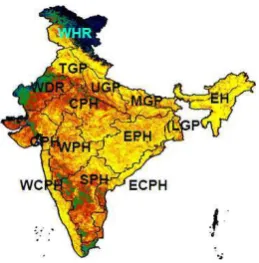
Figure 1: Study area with agro climatic region boundary (Agro climatic regions are: WHR: Western Himalayan Region, EH :Eastern Himalayan Region TGP: Transgangetic Plains, UGP: Upper Gangetic Plains, MGP: Middle Gangetic Plains, LGP: Lower Gangetic Plains, WDR: Western Dry Region, GPH: Gujarat Plains & Hills, CPH: Central Plateau & Hills, EPH: Eastern Plateau & Hills, WPH: Western Plateau & Hills , SPH: Southern Plateau & Hills, ECPH: East Coast Plains & Hills,WCPH:West Coast Plains & Hills).
From the global product of MODIS, India was extracted. The boundary of ACR was prepared through onscreen digitization and laid over Indian region to demarcate the different ACRs. After generating all the parameters during June to September from 2003-2012, all the ACR were masked out as the region of interest (ROI) using “ENVI image processing software” and information regarding all the parameters were retrieved separately for each ACR. Decadal mean and its standard deviation were computed for all the parameters for each month from each ACR in order to study the seasonal and inter annual variation.
3.5 Generation of coupling hot spots of LE
From the pixel based knowledge of all the parameters, a hierarchical decision rule algorithm was developed. Pixel wise information of the spatiotemporal behavior of the parameters (EF, SWI, Ts, Ta) were correlated with the LE dynamics. Lower values of LE found corresponding with the lower values of EF and SWI, and higher values of Ts and Ta. While studying the seasonal dynamics of the parameters during June to September, June month was found to be the hottest month with highest Ts and Ta along with lowest LE, EF and SWI. Spatiotemporal dynamics of the pixel information of the parameters were incorporated into a knowledge based classification scheme and thresholds were developed for each class that could able to classify the ACRs from lowest to moderate to high rainfall zones based on LE couplings with terrestrial and meteorological parameters from June to September during 2003-2012.
4 RESULTS
4.1. Long-term analysis of hydrological parameters
Hydrology of the study area was assessed by the seasonal total (June-September) rainfall obtained from IMD and seasonal average (June-September) ET obtained from MODIS ET during 2003-2011 in 14 agro climatic regions of India (Figure 2).
Figure 2: Long-term hydrological pattern in different ACR in India a) Total seasonal rainfall; b) Seasonal average ET.
The hydrological pattern could able to identify the study area categorically into low to moderate to high rainfall zones. The long term analysis of rainfall and ET showed similar behavior in spatial scale with little variation in temporal scales. Among the ACRs, the highest rainfall (>1500 mm) was observed in WCPH followed by EH (1000-2000 mm) corresponding to highest ET (>100 mm/month) and lowest rainfall was observed in WDR (100-400 mm) corresponding to lowest ET (15 - <40 mm/month). In the WHR, due to the unavailability of ET data, the accuracy of ET estimation was poor although the value was found somewhat matching with the rainfall information. Both gangetic plains and hills regions, and the plateau and hills regions, moderate rainfall
was observed with large variability (500 > RF <1300 mm; 20 > ET <90 mm/month).
ET is a direct input to the rainfall. Figure 3 depicts the seasonal variability (June-September) of annual mean and standard deviation of MODIS ET during 2003-2011. It is obvious that in June, the ET was less. The ET was high in July and August and slightly reduces in September. In the standard deviation images from June to September, it was observed that in the low rainfall areas, the standard deviation was found to be lower in June and as the monsoon progresses, those areas tend to show large deviation from the mean ET. That means the ET variability is lower in the arid region at the initial phase of monsoon and tends to increase with the availability of rainfall.
Figure 3: Seasonal distribution of actual MODIS ET a) Mean ET (Mean was computed from 2003-2011 for each month) ; b) Standard deviation of ET
On monthly to seasonal scales, land surface feedback to ET is dominated by soil moisture (here it is represented by SWI), which determines both surface evaporation and plant transpiration as plant growth is constrained by the soil moisture availability (Nemani et al., 2003). MODIS derived pixel wise seasonal transition of mean SWI (2003-2011) is depicted in Figure 4, which reveals the availability of soil moisture at different locations for ET during June to September.
Figure 4: Seasonal distribution of MODIS derived mean SWI (Mean was computed from 2003-2011 for each month)
From the spatial and temporal distribution of ET and SWI, the areas where both these values are low show the dry conditions in the area. The WDR, the lowest rainfall area showed the lowest ET and SWI value whereas the WCPH and the Himalayan region (EH, WHR) showed the highest ET and SWI (Figures 3 and 4). Throughout June to September, the MODIS estimated SWI variability was not found much in the Himalayan region (WHR
a b
a
and EH) and WCPH as those areas are the high rainfall areas. Highest seasonal variability of SWI was observed in the EPH, GPH and SPH followed by the central part of India mostly in the CPH, WPH and gangetic plains and some variability was also observed in WDR.
All the three parameters such as rainfall, ET and SWI are the primary parameters describing the hydrology of an area. The soil moisture-ET-rainfall feedback and its associated variability are controlled by the surface energy fluxes, through which anomalies in rainfall can be identified in different locations.
4.2. Dynamics of surface fluxes, land surface and meteorological parameters
In the climate system, LE and EF are the fundamental components linking surface fluxes to the hydrological cycle. These components changes periodically due to the variation of the land cover changes, vegetation dynamics, surface radiation parameters and temperature. Therefore, in order to understand the coupling process, it is important to correlate the parameters that can describe the coupling “hotspots”, which indicates that there is a strong relationship between the parameters. The coupling “hotspots” tends to vary region-wise in a spatiotemporal domain due to the changes in the surface energy transfer processes from land to the atmosphere and causes variability in rainfall.
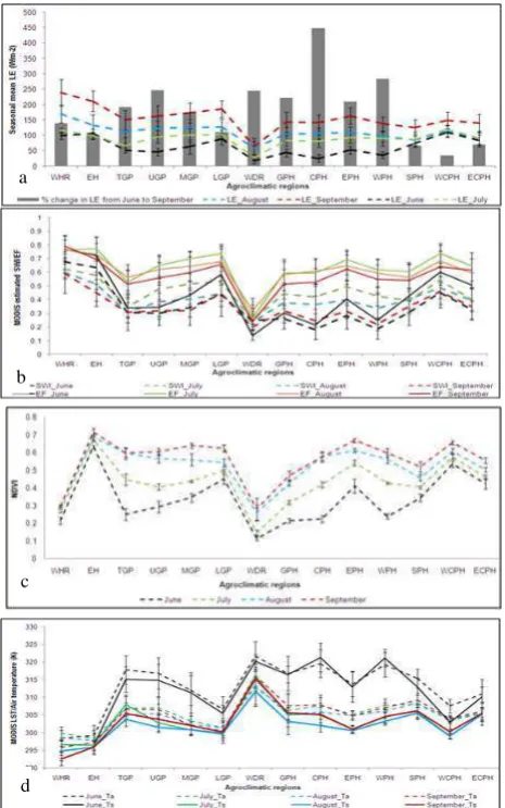
The seasonal dynamics (June to September) of the decadal mean (2003-2012) and standard deviation of the parameters e.g. LE, EF, SWI, NDVI, Ts and Ta are depicted in Figure 5. The spatial fluctuation of LE (Figure 5a) was found consistent with SWI and EF (Figure 5b) and NDVI (Figure 5c), whereas Ts and Ta showed opposite behavior (Figure 5d). Both SWI and EF are the direct positive input for LE and its associated variability over the land surface. Availability of soil moisture controls the partition of net radiation into sensible and latent heat flux, which changes significantly after the soil near the surface becomes wet enough due to rainfall. Due to the progress of rainfall from June onwards, a significant increase in LE was observed in all the sites (Figure 5a). The increase in LE from June to September with more than 220 Wm-2 was observed in the ACRs like UGP, WDR, GPH, CPH and WPH, where the seasonal variability in SWI was more. The lowest seasonal change in LE was found in WCPH where the seasonal variability of SWI was found negligible (as evident in Figure 4). Among the ACRs, during June to September, LE was found highest in WHR (90 Wm-2 ≥ LE< 300 Wm-2). In September, the maximum LE (>200 Wm-2) was observed in WHR. In that area, the SWI (>0.60) and EF (>0.70) were also found highest with lowest Ts (≤ 295 K) and Ta (≤ 297 k) although the NDVI was found lowest (<0.30). This is mainly due to the accumulated precipitation over snow covered surface that may lead to high SWI, hence, high EF and LE. Next to WHR, high LE was observed in EH and WCPH (90 Wm-2 ≥ LE<250 Wm-2) during June to September that were found corresponding well with the high values of SWI (0.4 ≥SWI≤ 0.9), EF (0.7≥EF≤ 0.9) and NDVI (EH: NDVI > 0.7; WCPH: NDVI >0.65). The lowest LE (20 Wm-2 <LE>70 Wm-2) was observed in WDR during June to September as this is an arid region with negligible rainfall (see Figure 2) with lowest values of SWI (<0.25), EF (<0.30) and NDVI (<0.30). Other ACRs showed moderate LE, SWI and EF
values with large variability. The seasonal dynamics of NDVI (Figure 5c), was found matching with LE for all the sites except WHR (where NDVI is not an inducing factor for rainfall to occur) and in rest of the ACRs, NDVI showed a major role for rainfall variation due to its consistent behavior with LE. Therefore, LE can be high either due to snow cover or vegetation growth.
Figure 5: Seasonal dynamics of terrestrial and meteorological Parameters in different ACR : a) LE ; b)SWI and EF; c) NDVI; d)LST and air temperature (Mean was computed from 2003-2012 for each month and error bars represents the standard deviation from mean).
Due to the predominant increasing in rainfall during July-September (varies widely in different ACR), caused the fall of both Ts and Ta (as depicted in Figure 5d) that lowered the sensible heat flux and also due to the increase of the surface humidity (as SWI and EF increased from July onwards) caused more LE fluxes to be transferred into the atmosphere by means of turbulent processes in land atmosphere interaction. The values of Ts and Ta were found decreased gradually from dry to wet months. The spatial pattern of both Ta and Ts were found similar in the ACRs and Ta was found almost 2K higher than Ts in all the sites throughout June to September. June showed the highest value of
a
b
c
d
both Ts and Ta for all the sites, the range varied from 296-322 K for Ts, the highest (>320 K) in WPH and WDR, and lowest in Himalayan region (≈ 296 K), whereas Ta varied from 298-322 K, the highest in WDR (>321 K) and lowest in WHR (≈ 298 K). The seasonal variation of EF and SWI in different ACR had shown opposite behavior as compared to temperature with the intensity of monsoon. Both Ts and Ta were found reducing with the increase of EF and SWI. Therefore, the temperature is negatively associated with the SWI and EF and hence, LE.
4.3 Prediction of coupling hotspots through LE fluxes
As observed from the earlier sections, hydrological parameters typically has wide variability from arid, semiarid to the Himalayan region, so are the turbulent energy fluxes such as LE, ET and EF. The predictability of the parameters can be further quantified with the statistical approach, where LE flux showed strong correlation with the terrestrial and meteorological parameters. To understand the degree of coupling at different ACRs, 2D scatter plots were drawn between LE versus various parameters (Figure 6).
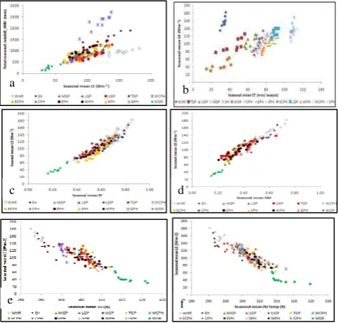
Figure 6: Scatter plot of MODIS derived LE (x-axis) versus parameters (y-axis), a) LE vs total seasonal rainfall; b) Seasonal mean LE vs seasonal mean ET; c) Seasonal mean LE vs seasonal mean EF; d) Seasonal mean LE vs seasonal mean SWI; e) Seasonal mean LE vs seasonal mean LST (Ts); f) Seasonal mean LE vs seasonal mean Ta. ; Seasonal mean was computed from June-September for each year.
Scatter plot (Figure 6a) between the total seasonal rainfall obtained from IMD versus seasonal mean LE estimated from MODIS (mean computed using observations from June to September) over the different ACRs was found to be positively linearly coupled with each other although R2 varies. This is attributed to the differences between the observed data as LE is from MODIS observations and rainfall data is from scattered ground station observation. The spatial fluctuations of the
parameters are mainly attributed to the variability of vegetation density, soil moisture and availability of rainfall. ACR wise separation was clearly evident along the linear line. But a mismatch in WHR between the IMD rainfall and MODIS estimated LE was observed. This is because IMD gridded rainfall data was obtained from the rain gauge stations, the density of which is not uniform throughout the Indian region. The densities of the stations are lower in the northern parts of India and WHR has negligible stations (Rajeevan et al., 2005). The regions such as WCPH and EH were observed as high rainfall areas (total seasonal rainfall ≥ 1500 mm) corresponding to highest LE (> 100 Wm-2). In the gangetic plains, and plateau and hills regions, large variability in the total seasonal rainfall was observed (500 mm < total seasonal rainfall<1300 mm) and those areas were found corresponding to large LE variability (77 Wm-2<LE≥122 Wm-2). WDR was observed as the lowest rainfall areas (total seasonal < 500 mm) corresponding to the lowest LE (LE ≤ 60 Wm-2). The deviation of data points within a given cluster was found mainly due to the annual variation of rainfall.
The scatter plot of MODIS derived LE versus ET (Figure 6b) was found to be positively linearly coupled with each other (0.71 < R2
≤ 0.91). Here also, a mismatch in WHR was observed. This is due to unavailability of data in this region as observed in MODIS ET product (see figure 2). WCPH and EH were observed as the high rainfall areas with highest value of both LE and ET and WDR showed as the lowest value of both LE and ET.
Both LE and EF are the terrestrial links to the atmosphere and when they are positively correlated with each other and also with soil moisture then a positive feedback of rainfall occurs. This feedback is highly variable in spatial and temporal domain. EF, which is the dimensionless fraction of available energy at the surface, is transmitted to the atmosphere through LE. Hence, the relationship of LE and EF is important to understand the possibility of rainfall and its anomaly in different locations. Scatter plot of MODIS derived LE versus EF (Figure 6c) showed a strong linear positive coupling (0.79 ≤ R2 ≤ 0.96). LE versus EF
coupling at spatial and temporal scales enables to discriminate the high and low rainfall zones. Overlapping of the cluster data points was observed with EF between 0.50 to 0.72 and LE between 80 to 130 Wm-2 and was noticed mostly in the gangetic plains and plateau and hills regions, whereas the Himalayan region (WHR and EH) and WCPH (LE > 100 Wm-2 and EF > 0.6) as well as arid region (WDR) (LE ≤ 60 Wm-2 and EF ≤ 0.32), showed a clear demarcation of the area with excessive and deficient rainfall respectively.
The variability of soil moisture, which has a direct input to the LE and EF, strongly influence convective processes of precipitation. The 2D scatter plot (Figure 6d) of MODIS derived LE versus SWI showed strong positive correlation with significant positive linear increase (0.80 ≤ R2 ≤ 0.93) with some deviation of the data points from given cluster in a zone that is attributed to the variation in the annual rainfall pattern. The sensitivity of LE to SWI found varying from arid, semi arid to the Himalayan region. Except WDR (lowest SWI; SWI < 0.3) and Himalayan region (highest SWI; SWI ≥ 0.5), the other areas showed overlapping where the LE found varying from 80 to 140 Wm-2 and SWI found varying from 0.25 to 0.55.
a
b
c d
The 2D scatter plots of MODIS derived LE versus Ts (Figure 6e) and MODIS derived LE versus Ta (Figure 6f) showed increasing LE with decreasing Ts and Ta. A clear demarcation between the highest rainfall (Himalayan region; Ts ≤ 298 K; Ta < 305 k) and the lowest rainfall (WDR; Ts > 312 K; Ta > 314 k) were observed. Overlapping of cluster of data points were observed in moderate to low rainfall areas (300 k < Ts≤ 310 K; 302 K< Ta≤ 314 K). The statistical relationships among the parameters with R2 values are explained in table 2.
4.4 Seasonal variation of coupling hotspots of LE
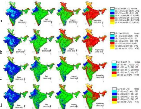
Based on the LE couplings with various parameters, India as a whole was categorized in to different rainfall zones such as zone 1: lowest rainfall, zone 2: low rainfall, zone 3: moderate rainfall; zone 4: moderate to high rainfall; zone 5: very high rainfall, zone 6: highest rainfall. The pixel-by-pixel segmentation of annual mean (2003-2012) of seasonal dynamics of LE coupling hotspots are depicted in Figure 7.
Figure 7: Seasonal coupling of LE versus land surface and meteorological parameters (decadal mean were computed from 2003-2012 for the all the parameters). a. LE vs EF; b. LE vs SWI; LE vs Ts; LE vs Ta. Different rainfall zones are: LTRZ: Lowest rainfall zone; LRZ: Low rainfall zone; MRZ: Moderate rainfall zone; HRZ: High rainfall zone; VHRZ: Very high rainfall zone; HTRZ: Highest rainfall zone;
The above couplings explained the roles of soil moisture and temperature in surface energy exchange processes. Higher LE class was found corresponding to the high EF, high SWI and low Ts and Ta. The shift in rainfall zones were found varying from dry
to wet months with the increase in LE, EF and SWI as these parameters provide positive feedback to rainfall and decrease of Ts and Ta, as they provide negative feedback to rainfall.
The transition of agro climatic zone wise availability of rainfall from June to September along with the surplus and deficient rainfall areas can very well understood from the seasonal dynamics of LE coupling hotspots and this also shows that in India, June is comparatively drier month with low crop cover (low NDVI), low soil moisture (low SWI), high temperatures (Ts and Ta) (see Figure 5) which are the constraint for ET to take place (it is obvious from the June ET in Figure 2). Hence, both LE and EF were found lowest during June. Both LE versus EF and LE versus SWI coupling hotspots increased linearly as the rainfall progresses with highest value in September. Throughout June to September, LE coupling hotspots with high rainfall (high LE versus high EF; high LE versus high SWI) were observed in the WCPH and Himalayan region (WHR and EH), followed by the gangetic plains (regions were showing as decreasing pattern of LE coupling hotspots i.e. LGP>MGP>UGP>TGP), EPH and ECPH. LE coupling hotspots with low rainfall was observed in WDR followed by WPH and CPH. It is understood from the previous sections that both Ta and Ts lowers down as rainfall progresses. Figures 7c and 7d show the LE versus Ts and LE versus Ta coupling hotspots over different ACR. In the month of June, highest Ta and Ts were found coupled with the lowest LE values and with the progress of rainfall, the coupled relationships tend to change where the LE found increased gradually with decreased Ta and Ts. The seasonal transition of temperature (Ts and Ta) in both humid regions and arid regions became unaffected as negligible temperature difference was observed in those areas whereas in other regions both the temperatures dropped down drastically in the month of July due to frequent rainfall and it remained almost unchanged till September. The higher temperature difference more than 10 K from June to July was observed in the sites such as TGP, UGP, GPH, CPH, WPH (both Ta and Ts) and MGP, EPH (only Ts). In contrast with the bare soil, the dense vegetation has relatively higher LE, EF and SWI values, usually LE on the order of 200-300 W·m−2 and EF in the range of 0.6-0.7. The sparse vegetation has very low values with LE usually less than 80 Wm−2 and EF less than 0.42.
5. CONCLUSIONS
The present study very well explained methodology to understand and map LE coupling hotspots using multi-year (2003-2012) MODIS observed LE flux versus land surface and meteorological parameters over Indian region. Based on the LE couplings, different agro climatic zones were categorized into various rainfall zones i.e. from highest to lowest. Seasonal variations in the LE coupling hotspots are observed that are believed to be strongly associated with the land surface and meteorological parameters. LE hotspots showed wide variability in spatiotemporal domain in both locations and intensity, demonstrating different responses of individual land surfaces to LE dynamics. Both soil moisture and temperature were found to be the important indicators of rainfall and its variability in surface energy exchange processes. Higher LE class was found corresponding with the high EF, high SWI and low Ts and Ta. The statistical analysis showed that the parameters could be strongly coupled well with each other depicting a clear demarcation Table 2: R2 values of LE versus parameters obtained in 2D
scatter plot.
a
b
c
d
between lowest and highest rainfall zone. This indicates that this coupling process can able to capture reasonably the spatial distribution of rainfall over India. This is an important input for climatological and hydrological modeling for predicting rainfall in a particular area.
6. ACKNOWLEDGEMENTS
The study was carried out under the Project funded by the Department of Science and Technology, New Delhi under Women Scientist Scheme (WOS-A) is gratefully acknowledged. The author is also grateful to the Director, DAIICT, Gandhinagar for providing necessary infrastructure for carrying out the research work. The author also acknowledges Prof R Ghosh for his moral support and encouragement.
REFERENCES
Bastiaanssen, W.G.M., Menenti, M., Feddes, R.A. and Holstlag, A.A.M., 1998. A remote sensing surface energy balance algorithm for land (SEBAL) 1: Formulation. Journal of Hydrology, 213, pp. 198–212.
Bhattacharya, B.K., Mallick, K., Patel, N.K. and Parihar, J.S., 2010. Regional clear sky evapotranspiration over agricultural land using remote sensing data from Indian geostationary meteorological satellite. Journal of Hydrology, 387, pp. 65–80.
Campbell, G.S and Norman, J.M., 1998. An Introduction to Environmental Biophysics. Springer, New York, pp. 286.
Cano, D., Monget, J.M., Albuisson, M., Guillard, R., Regas, N. and Wald, L., 1986. A method for the determination of the global solar radiation from meteorological satellite data. Solar Energy, 37, pp. 31–39.
Carlson, T. N., R. R. Gillies, and T. J. Schmugge, 1995. An interpretation of methodologies for indirect measurement of soil water content, Agriculture and Forest Meteorology, 77, pp. 191– 205, 1995.
Choudhury, I and Ghosh, R., 2014. Spatiotemporal coupling of land surface and energy balance parameters with monsoon rainfall using remote sensing technology. International Journal of Remote Sensing, 35 (2), pp. 532–553.
Guo, Z. et al., 2006. GLACE: The Global Land-Atmosphere Coupling Experiment. 2. Analysis. J. Hydrometeor., 7, pp. 611-625.
Koster, R. D. et al., 2004. Regions of strong coupling between soil moisture and precipitation. Science, 305, pp.1138-1140.
Mallick, K., Bhattacharya, B.K., Rao, V.U.M., Reddy, D.R., Banerjee, S., Hoshali, V., Pandey, V., Kar, G., Mukherjee, J., Vyas, S.P., Gadgil, A.S. and Patel, N.K. 2009. Latent heat flux estimation in clear sky days over Indian agro ecosystems using noontime satellite remote sensing data. Agricultural and Forest Meteorology, 149 (10), pp. 1646–1665.
Nishida, K., Nemani, R.R., Running, S.W., Glassy, J.M., 2003. An operational remote sensing algorithm of land surface vaporation. Journal of Geophysical Research, 108 (D9), pp.4270.
Rajeevan, M., J., Bhate, J., D. Kale, and B. Lal., 2005. Development of High Resolution Daily Gridded Rainfall Data for the Indian Region. Report Met. Monograph Climatology No. 22/2005, National Climate Centre, Indian Meterological
Department, Pune, India.
(ftp://squall.met.fsu.edu/LAU/070108_1446/doc/ref_report.pdf)
Rajeevan, M., J., Bhate, J., D. Kale, and B. Lal., 2006. High Resolution Daily Gridded Rainfall Data for the Indian Region:Analysis of Active and Break Monsoon Spells. Current Science, 91(3), pp.296-306.
Roerink, G.J., Su, Z. and Menenti, M., 2000. S-SEBI: a simple remote sensing algorithm to estimate the surface energy balance. Physics and Chemistry of the Earth, 25, pp. 147-157.
Sandholt, I., K. Rasmussen, and J. Andersen. 2002. A Simple index for natural surfaces. International Journal of Remote Sensing, 14, pp. 1119–1131
Components Set of Equations; Computational methods & Reference