USING MCSST METHOD FOR MEASURING SEA SURFACE TEMPERATURE WITH
MODIS IMAGERY AND MODELING AND PREDICTION OF REGIONAL VARIATIONS
WITH LEAST SQUARES METHOD (CASE STUDY: PERSIAN GULF, IRAN)
M. S. Pakdamana *, S. Eyvazkhanib, S. A. Almodaresic, A. S. Ardekanic, M. Sadeghnejad c, M.Hamisid
a Dept. of GIS and Remote Sensing Engineering, Islamic Azad University, Yazd Branch [email protected]
bDept. of Industrial Engineering, Iran University of Science and Technology
c Dept. of GIS and Remote Sensing Engineering, Islamic Azad University, Yazd Branch d Dept. of Information Technology, Shiraz University
KEY WORDS: Thermal Remote Sensing, MCSST, MODIS, Modeling, Least Squares, Persian Gulf
ABSTRACT:
Nowadays, many researchers in the area of thermal remote sensing applications believe in the necessity of modeling in environmental studies. Modeling in the remotely sensed data and the ability to precisely predict variation of various phenomena, persuaded the experts to use this knowledge increasingly.Suitable model selection is the basis for modeling and is a defining parameter. So, firstly the model should be identified well. The least squares method is for data fitting. In the least squares method, the best fit model is the model that minimizes the sum of squared residuals. In this research, that has been done for modeling variations of the Persian Gulf surface temperature, after data preparation, data gathering has been done with multi-channel method using the MODIS Terra satellites imagery. All the temperature data has been recorded in the period of ten years in winter time from December 2003 to January 2013 with dimensions of 20*20 km and for an area of 400 km2. Subsequently, 12400 temperature samples and variation trend control based on their fluctuation time have been observed. Then 16 mathematical models have been created for model building. After model creation, the variance of all the models has been calculated with ground truth for model testing. But the lowest variance was in combined models from degree 1 to degree 4. The results have shown that outputs for combined models of degree 1 to degree 3 and degree 1 to degree 4 for variables does not show significant differences and implementation of degree 4 does not seem necessary. Employment of trigonometric functions on variables increased the variance in output data. Comparison of the most suitable model and the ground truth showed a variance of just 1⁰. The number of samples, after elimination of blunders reduced to 11600 samples. After this elimination, all the created models have been run on the variables. Also in this case, the highest variance has been obtained for the models that have trigonometric functions for variables. The lowest variance has been obtained for combined models of degree 1 to 3 and 4. After the elimination of the blunders and running the model once more, the variance of the most suitable model reached to 0.84⁰. Finally, among the 16 models, 13 models showed less than 1⁰ that demonstrates the accuracy of the selected models for scrutiny and predict variations of the surface temperature in this area.
1. INDTODUCTION
Nowadays, reduce the boundaries between of various Science with progress of new technology. This is obvious to everyone that use of technical and mathematical science in Earth and Environmental science. Remote Sensing having ability for improvement of science purpose as a semi-environmental and semi-technical Knowledge. Sea Surface temperature (SST) is the most important ocean parameters that effective on atmospheric systems, climate and aquatics life. The Variations of sea surface temperature, playing main role in energy exchange and momentary changing of water vapour between ocean and atmosphere. Also, SST is a main parameter for prediction of climatology models(Vigan, et al, 2000).
Air masses in the Earth's atmosphere are highly modified by sea surface temperatures within a short distance of the shore. Localized areas of heavy snow can form in bands downwind of warm water bodies within an otherwise cold air mass. Warm sea surface temperatures are known to be a cause of tropical cyclogenesis over the Earth's oceans.
Tropical cyclones can also cause a cool wake, due to turbulent mixing of the upper 30 meters (100 ft) of the ocean. SST changes
* Corresponding Author
diurnally, like the air above it, but to a lesser degree due to its higher specific heat. In addition, ocean currents and the global thermohaline circulation affect average SST significantly throughout most of the world's oceans.
For SST's near the fringe of a landmass, offshore winds cause upwelling, which can cause significant cooling, but shallower waters over a continental shelf are often warmer. Its values are important within numerical weather prediction as the SST influences the atmosphere above, such as in the formation of sea breezes and sea fog. It is also used to calibrate measurements from weather satellites (Luyten et al 1999).
For this reasons, Identified the Importance of Awareness from trend of SST changes in a regions, More than ever. We must use a appropriate model for predication trend of SST changes. Models in used the resulting from check trend of SST changes in the past. SST data gathering is very costly and very time-consuming in classical method. One of the applications of remote sensing and satellite imagery, SST data gathering with fewer cost and more accurate. In this paper, investigate Sea surface temperature (SST) with fusion of Remote sensing technology and mathematical modeling. Thereby, produce thermal data with use Terra-MODIS sensor images and MCSST method and prepare
temperature changing model with use least squares method in region of interest.
1.1 Area of Study
The Persian Gulf is located in Western Asia between Iran and the Arabian Peninsula (Figure 1). The small freshwater inflow into the Persian gulf is mostly from the Tigris, Euphrates, and Kārūn rivers. Surface-water temperatures range from 75 to 90 °F (24 to 32 °C) in the Strait of Hormuz to 60 to 90 °F (16 to 32 °C) in the extreme northwest. These high temperatures and a low influx of fresh water result in evaporation in excess of freshwater inflow; high salinities result, ranging from 37 to 38 parts per thousand in the entrance to 38 to 41 parts per thousand in the extreme northwest. Even greater salinities and temperatures are found in the waters.
Figure 1. Persian Gulf location and area of interest
2. MATERIALS AND METHODS
How do climate changing in various conditions? This hypothesis considered in climate concerning long times. variations of SST is one of this climate changing parameters. Variations of SST, is not uniform in various regions of Hydrosphere and local changing is quite depended on local Climatic parameters. In this research, that has been done for modeling variations of the Persian Gulf surface temperature of the period of ten years in winter time from December 2003 to January 2013.
2.1 Modis Sensor
MODIS (or Moderate Resolution Imaging Spectroradiometer) is a key instrument aboard the Terra (EOS AM, launched on 18 December 1999) and Aqua (EOS PM, launched on 4 May 2002) satellites. Terra's orbit around the Earth is timed so that it passes from north to south across the equator in the morning, while Aqua passes south to north over the equator in the afternoon. Terra MODIS and Aqua MODIS are viewing the entire Earth's surface every 1 to 2 days, acquiring data in 36 spectral bands, or groups of wavelengths between 0.405 and 14.385 µm, and it acquires data at three spatial resolutions -- 250m, 500m, and 1,000m. The MODIS instrument has a viewing swath width of 2,330 km. It was decided that to calculate the SST, used from this sensor’s images, According to Relatively broad coverage and Also Good temporal resolution and facilitating their accessibility of their sensor.
World maps of coverage and also temperature of water surface and land by using data from this sensor is achievable, According to wide spectral range and extensive coverage of MODIS images.
determination. Bands of particular utility to infrared SST determination are listed in Table 1.
Band Number Band Center (μ) Bandwidth (μ)
20 3.750 0.1800
22 3.959 0.0594
23 4.050 0.0608
31 11.030 0.5000
32 12.020 0.5000
Table 1. Bands for MODIS Infrared SST Determination
2.2 Data used
For this research, all the SST data has been recorded in the period of ten years in winter time from December 2003 to January 2013 [Table 2] with dimensions of 20*20 km and for an area of 400 km2. Subsequently, 12400 SST samples and variation trend control based on their fluctuation time have been observed.
date date date date
Table 2. Data Collection from MODIS sensor
2.3 Calculation SST with MCSST method
An angular-dependent split-window equation is proposed for determining the Sea Surface Temperature (SST) at any observation angle, including large viewing angles at the image edges of satellite sensors with wide swaths (Raquel, 2006). MCSST is one of the methods in this algorithms that base on Radiance reduce the amount of atmospheric absorption dependent on Radiance difference at same time scan from a place but with two different wavelengths(Saradjian, M.R. and L.W.B. Hayes, 1993),( Otis B. Brown). Because different wavelengths have different atmospheric absorption. The following formula can be derived sea surface temperatures for MODIS sensor (Evans, R.H., 1999):
MODIS (MCSST) = c1+ (c2*T31) + (c3*(T31-T32)) + (c4*(sec (ө)-1)*(T31-T32)) (1) Where T31 & T32 refer to brightness temperature at bands 31 and 32 (11.03μm, 12.02μm), and θ is the zenith angle to the satellite radiometer measured at the sea surface and coefficients c1 to c4 are derived from radiative transfer modeling.
Coefficients for the MODIS band 31 and 32 SST retrieval algorithm, derived using ECMWF or radiosondes, assimilation model marine atmospheres to define atmospheric properties and variability (Table 3 & 4).
T31-T32>0.7
Table 3. Coefficients for the MODIS Band 31 and 32 SST retrieval algorithm, derived using radiosondes to define
atmospheric properties and variability.
T31-T32>0.7
Table 4. Coefficients for the MODIS Band 31 and 32 SST retrieval algorithm, derived using ECMWF assimilation model
marine atmospheres to define atmospheric properties and variability.
2.4 Modeling with Least Squares method
Modeling has been a useful tool for engineering design and analysis. The definition of modeling may vary depending on the application, but the basic concept remains the same: the process of solving physical problems by appropriate simplification of reality.
The least square methods (LSM) is probably the most popular technique in statistics. This is due to several factors. First, most common estimators can be casted within this framework. For example, the mean of a distribution is the value that minimizes the sum of squared deviations of the scores. Second, using squares makes LSM mathematically very tractable because the Pythagorean theorem indicates that, when the error is independent of an estimated quantity, one can add the squared error and the squared estimated quantity. Third, the mathematical tools and algorithms involved in LSM (derivatives, eigen-decomposition, singular value decomposition) have been well studied for a relatively long time (Loewe, P.,2003).
The least-squares method is usually credited to Carl Friedrich Gauss (Björck, 1996). but it was first published by Adrien-Marie Legendre.
A mathematical procedure for finding the best-fitting curve to a given set of points by minimizing the sum of the squares of the offsets ("the residuals") of the points from the curve. The sum of the squares of the offsets is used instead of the offset absolute values because this allows the residuals to be treated as a continuous differentiable quantity. However, because squares of the offsets are used, outlying points can have a disproportionate effect on the fit, a property which may or may not be desirable depending on the problem at hand.
Vertical least squares fitting proceeds by finding the sum of the squares of the vertical deviations R2 of a set of ‘n’ data points from a function.
= ∑[ �− � �, , , … , � ]
Note that this procedure does not minimize the actual deviations from the line (which would be measured perpendicular to the given function). In addition, although the unsquared sum of distances might seem a more appropriate quantity to minimize, use of the absolute value results in discontinuous derivatives which cannot be treated analytically. The square deviations from each point are therefore summed, and the resulting residual is then minimized to find the best fit line. This procedure results in outlying points being given disproportionately large weighting. The condition for R2 to be a minimum is that:
These lead to the equations:
+ ∑ �
After observing the annual variations, 16 mathematical models have been created for model building [Table 5]. After model creation, the variance of all the models has been calculated with ground truth for model testing. But the lowest variance was in combined models from degree 1 to degree 4. The results have shown that outputs for combined models of degree 1 to degree 3 and degree 1 to degree 4 for variables does not show significant differences and implementation of degree 4 does not seem necessary. Employment of trigonometric functions on variables increased the variance in output data. Comparison of the most suitable model and the ground truth showed a variance of just 1⁰. Finally, because of the less complexity and fewer variance, we select model no.7 and compare model outputs with SST data in MCSST method [Figure 2]. International Archives of the Photogrammetry, Remote Sensing and Spatial Information Sciences, Volume XL-1/W3, 2013
7 1.006696681475738
Table 5. Models form and their variance
Where: M= month Y=Year
y=SST based on output model no. 7
Figure 2. Compare model no. 7 outputs with SST data in MCSST method, where blue line is MCSST data and red line is
output model
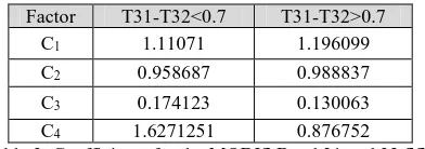
The number of samples, after elimination of blunders reduced to 11600 samples. After this elimination, all the created models have been run on the variables. Also in this case, the highest variance has been obtained for the models that have trigonometric functions for variables. The lowest variance has been obtained for combined models of degree 1 to 3 and 4. After the elimination of the blunders and running the model once more, the variance of the most suitable model reached to 0.84⁰ in models no. 7 & 16. Finally, among the 16 models, 13 models
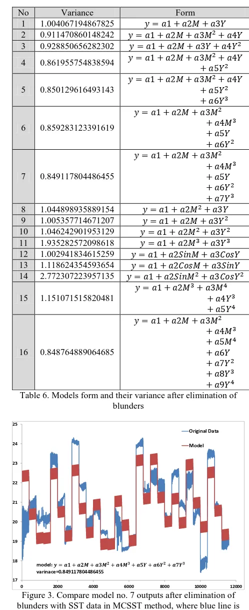
showed less than 1⁰ that demonstrates the accuracy of the selected models for scrutiny and predict variations of the surface temperature in this area [Table 6] & [Figure 3].
No Variance Form
Table 6. Models form and their variance after elimination of blunders
Figure 3. Compare model no. 7 outputs after elimination of blunders with SST data in MCSST method, where blue line is
MCSST data and red line is output model
Where: M= month Y=Year
y=SST based on output model no. 7 17
0 2000 4000 6000 8000 10000 12000
Original Data
0 2000 4000 6000 8000 10000 12000
Original Data
Model
model:
varinace=0.849117804486455
3. CONCLUSIONS
Considering the importance of modeling in remote sensing, in this research, we use Least Squares Method (LSM), In order to evaluate the SST variations of Persian Gulf surface.
The results indicated that, employment of trigonometric functions on variables increased the variance in output data and lowest variance has been obtained for combined models of degree 1 to 3 and 4.
REFERENCES
Raquel, N., 2006. An angular-dependent split-window equation for SST retrieval from off-nadir observations. 1-4244-1212-©2007 IEEE.
Björck, A., 1996. Numerical Methods for Least Squares Problems. SIAM. ISBN 978-0-89871-360-2.
Kenney, J. F. and Keeping, E. S. 1962 "Linear Regression and Correlation." Ch. 15 in Mathematics of Statistics, Pt. 1, 3rd ed. Princeton, NJ: Van Nostrand, pp. 252-285.
Saradjian, M.R. and L.W.B. Hayes, 1993, Automated pattern recognition of rotated sea surface temperature featuresusing sequential satellite images, Proceedings of the International Geoscience and Remote Sensing Symposium (IGARSS' 93), Tokyo, Japan, pp.1827-1829.
Otis B. Brown, Peter J. Minnett, R. Evans, E. Kearns, K. Kilpatrick, A. Kumar, R. Sikorski & A. Závody, MODIS Infrared Sea Surface Temperature Algorithm (Algorithm Theoretical Basis Document Version 2.0),University of Miami
Vigan, X, Provost, C, Bleck, R, Courtier, P, 2000, Sea surface velocities from Sea Surface Temperature image sequences, Journal of Geophysical Research.
Evans, R.H., 1999. Processing Framework and Match-up Database MODIS algorithm (V3)
http://modis.gsfc.nasa.gov/data/atbd/atbd_mod26.pdf, University of Miami.
Loewe, P.,2003. Weekly North Sea SST Analysis since 1968. Original digital archive held by Bundesamt für Seeschifffahrt und Hydrographie, D-20305 Hamburg, P.O.Box 301220, Germany
Luyten P.J., Jones J.E., Proctor R., Tabor A., Tett P. and Wild-Allen K., 1999. COHERENS – A Coupled Hydrodynamical-Ecological Model for Regional and Shelf Seas: User Documentation. MUMM report, Management Unit of the Mathematical Models of the North Sea, 914 pp.
[Available on CD-ROM at http://www.mumm.ac.be/coherens]