EXTRACTING LANE GEOMETRY AND TOPOLOGY INFORMATION FROM VEHICLE
FLEET TRAJECTORIES IN COMPLEX URBAN SCENARIOS USING A REVERSIBLE
JUMP MCMC METHOD
O. Roetha,∗, D. Zaumb, C. Brennerc
a
Corporate Research, Robert Bosch GmbH Hildesheim, Germany - [email protected] b
Chassis Systems Control, Robert Bosch GmbH Hildesheim, Germany - [email protected] c
Institute of Cartography and Geoinformatics, Leibniz Universit¨at Hannover, Germany - [email protected]
KEY WORDS:Lane Accurate Map Construction, Trajectories, GPS, DGPS, IMU, Road Network, Reversible-Jump Markov chain Monte Carlo
ABSTRACT:
Highly automated driving (HAD) requires maps not only of high spatial precision but also of yet unprecedented actuality. Traditionally small highly specialized fleets of measurement vehicles are used to generate such maps. Nevertheless, for achieving city-wide or even nation-wide coverage, automated map update mechanisms based on very large vehicle fleet data gain importance since highly frequent measurements are only to be obtained using such an approach. Furthermore, the processing of imprecise mass data in contrast to few dedicated highly accurate measurements calls for a high degree of automation.
We present a method for the generation of lane-accurate road network maps from vehicle trajectory data (GPS or better). Our approach therefore allows for exploiting today’s connected vehicle fleets for the generation of HAD maps. The presented algorithm is based on elementary building blocks which guarantees useful lane models and uses a Reversible Jump Markov chain Monte Carlo method to explore the models parameters in order to reconstruct the one most likely emitting the input data. The approach is applied to a challenging urban real-world scenario of different trajectory accuracy levels and is evaluated against a LIDAR-based ground truth map.
1. INTRODUCTION
Technologies for autonomous vehicles (AV) and advanced driver assistance systems (ADAS) are topics which are intensively in-vestigated by many automotive OEMs and suppliers. While a lot of upcoming function of AV and ADAS are heavily related to a high accurate map (HAM) the challenges of map generation become one of the main fields of interest but remain partially un-solved so far. As a promising technique, crowd-sourcing methods are in the limelight of many works concerned with fully auto-mated map construction.
This paper presents a new approach for extending a street ac-curate road network map to a lane acac-curate one using trajecto-ries of GPS-monitored vehicle fleets. Reversible Jump Markov chain Monte Carloand simulated annealing are used to explore the valid dimensions and configurations of a model representing the lane graph to reach the one which most probably emitted the input data.
The paper is organized as follows: Section 2 outlines the state of the art of lane accurate road network generation. Section 3 intro-duces the mathematical basics needed in our approach. Section 4 presents the basic models which are used by our subsequently de-scribed lane accurate map generation algorithm. Section 5 details the input data, namely the trajectory fleet measurement data in three accuracy levels and a LIDAR based ground truth map of an exemplary scenario. Finally, the results of our approach evaluated against the ground truth map are presented. Section 6 concludes the paper and presents possible future work.
∗Corresponding author
2. STATE OF THE ART
Since GPS is publicly available, various approaches for the fully automated derivation of road network graphs from vehicle fleet trajectories have been presented. This section gives an overview of the state of the art of road and lane accurate map construction in 2.1 and 2.2 respectively.
2.1 Road Accurate Map Construction
Since our approach of lane accurate map construction presented in Section 4 is inseparable from the topic of road accurate map construction we will first present the state of the art with re-spect to the latter. To overcome the great diversity of approaches Ahmed et al. (2015) introduced a categorization in three classes: A) intersection linking, B) incremental track insertion and C) point clustering. Algorithms of category A firstly transfer detected curves and intersections into nodes in the graph and, secondly, analyze the trajectories to identify the connections be-tween nodes. This technique is used with remarkable results by Karagiorgou and Pfoser (2012). Incremental track insertion algo-rithms insert the trajectories to an empty map iteratively and up-date the resulting graph at each iteration by using map matching procedures. Finally, point clustering approaches as used by Bia-gioni and Eriksson (2012) transform the input data into a point cloud to subsequently cluster them for example into a density based discretization image to identify the original graph.
2.2 Lane Accurate Map Construction
The categorization from Section 2.1 applies for lane accurate map construction. Bruntrup et al. (2005) provide a generic approach as a representative of the incremental track insertion algorithm. Their system uses AI techniques for inferring the geometries and
This contribution has been peer-reviewed. The double-blind peer-review was conducted on the basis of the full paper.
a cluster algorithm to generate the road map. As an intersec-tion linking algorithm Schroedl et al. (2004) present an approach which firstly divides the input in roads and intersections in order to infer the roads and subsequently the lanes centerlines for each portion.
3. MATHEMATICAL BASICS
In this section the mathematical basics of our approach are sum-marized. Section 3.1 comprises the basic idea ofMarkov chain Monte Carlo(MCMC) methods which constitutes the principle of the subsequently presentedReversible Jump MCMCmethods (Section 3.2).
3.1 Markov chain Monte Carlo Methods
Monte Carlomethods are statistical algorithms which can be used e.g. for the computation of large hierarchical models by generat-ing representative random samples from the investigated function or numerical approximations of integrals.
While there are different approaches to sample from low - dimen-sional spaces likeImportance Sampling(Hastings, 1970),Markov chain Monte Carlomethods enable sampling from arbitrarily com-plex distributions out of high - dimensional spaces. The main idea of MCMC methods is to define a transition kernelT of a chain which has the investigated functionπas its stationary distribution which can then be used to generate a sample.
A general MCMC method is theMetropolis-Hastings-Algorithm (MH) (Hastings, 1970)(Metropolis et al., 1953). It generates a possible new stateθ′of the Markov chain from a proposal distri-butionq(·|θ)and decides whether or not to accept it. This proce-dure is hereafter referred to asMH step. If thedetailed balance condition
T(θ′|θ)π(θ) =T(θ|θ′)π(θ′)
is satisfied, a stationary distribution exists and if the generated chain stays irreducible and aperiodic (Meyn and Tweedie, 1993) the chain converges to this distribution. The probability of ac-cepting the new state is defined as
θ(t+1)=
Since the convergence requirements are fulfilled,πis the station-ary function of the transition kernelT(θ(t+1)|θ(t)).
3.2 Reversible Jump Markov chain Monte Carlo Methods
MCMC methods are limited to problems of fixed dimension. In order to enable dimension changes ofθ, Green introduced the Re-versible Jump MCMC(rjMCMC) methodology in (Green, 1995). This method extends the general MCMC methods by transitions in the kernelTbetween different state spaces.
LetSkbe thek-th state space andπkthe target distribution
de-fined on thek-th space. The combined state space of the disjunct spaces is defined as
S=∪Kk=1({k} ×Sk)
where the stateθ ∈ Skfrom thek-th space is written as(k, θ).
The transition kernel onSwithin each subspace is defined as
T((k′, θ′)|(k, θ)) =
Tk ifk=k′(Section 3.1)
0 else .
Additionally to the transitions within a spaceSk, inter-space
tran-sitions fromSi to Sj can be implemented by defining a joint
spaceS′where the spaces are complemented by additional com-ponents so as to have the same dimension:
S′= ({i} ×Si×Ui)∪({j} ×Sj×Uj)
The needed complementing components U are sampled from
ui∼qi(·|θi). If such a transition is chosen,uiis drawn and the
transition(θj, uj) = τ(θi, ui)to the new state(kj,(θj, uj))is
evaluated and accepted with probability
(k(t+1), θ(t+1)) =
(kj, θj) ifw≤b((ki, θi),(kj, θj))
(ki, θi) else
w∼Uniform[0,1].
The detailed balance condition must still be satisfied forb(·,·)to ensure thatπbecomes the Markov chains stationary distribution. This requires the following consideration:
Φ(Θi,Θj) =pi·πi(θi)·qi(ui|θi)
Φ(Θj,Θi) =pj·πj(θj)·qj(uj|θj)· |Jτ|i| (2)
withJτ|i=
∂τ(θi, ui)
∂(θi, ui)
are the probabilities of switching between the spaceSiand Sj
andpi/pjare those of choosing this move. The probabilities are
defined on the same space
Rdim(Si)+dim(Ui)=Rdim(Sj)+dim(Uj)
but in different variables. Thus, according to the transformation theorem in (2) the determinant of the Jacobian ofτis multiplied to scale the equations right.
According to (1) the acceptance probability of the transition is
b((ki, θi),(kj, θj)) =
used to describe a lane accurate road and, subsequently, the con-struction algorithm is explained in detail in Section 4.2.
4.1 Model
The models described in the following are able to map a general traffic situation on lane level. To ensure that the models stay valid and realistic they are subjected to restrictions which are imposed by using a set of primitives and assembly rules. The overall model is split into two different types of submodels, namely streets and crossings which can be separated in the roadmap graph.
4.1.1 Street Model A street model is represented by a list of nodes of the underlying road map (see Fig. 1{S1, S2, S3}).
Any point along the road can be described by a parametrization valueυ ∈ [0.0,1.0]as it can be seen in Fig. 1. Based on the parametrization it is possible to defineblockson the road as it is exemplarily shown in Fig. 1 with a gray box which extends from the relative value0.6to0.8. Thus, the absolute extension in me-ters depends on the length of the road. A general block can then be specified using the following parameters:
• Number of lanes • Width of each lane
• Type of each lane marking (e.g. dashed, solid,...) • Middle gap separating the opposite directions • Curvature
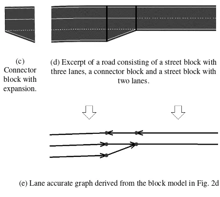
In our work two different types of blocks are used. Firstly, astreet blockdescribes a section with constant information regarding the number of lanes as it is shown in Fig. 2a and Fig. 2b. Secondly, aconnector blockextends the properties of a general block by a connection permutation which makes up the difference between two consecutive street blocks as it can be seen in Fig. 2c. Fig. 2d shows a composition of a street block with three lanes which merges into a street block with two lanes via a connector block. Finally, each block can be transformed into a graph representa-tion, e.g. Fig. 2e shows the lane graph of Fig. 2d.
Since a block has its curvature as a variable property, the models are not described by linear interpolations but by cubic Hermite splines (Catmull and Rom, 1974) to get a smooth and realistic representation of a road. The required values are the start- and the endpoint of the block and the gradients in these points are derived from the road accurate graph. The length of the gradient vectors influences the form of the block.
0.0
1.0 0.6 - 0.8
S1
S2
S3
Figure 1. An exemplary street model referenced to{S1, S2, S3}
of the road accurate map and an exemplary block spanning from the relative value0.6to0.8. The filled bullets mark nodes and
the arrows mark edges of the road accurate graph.
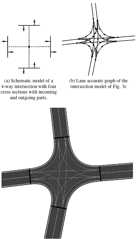
4.1.2 Crossing Model A crossing model consists of an ac-cessible area (asphalt) and connection lanes. It is defined by a centroid point equivalent to the intersection node(s) of the road accurate graph. Each attached road is connected by a cross sec-tion with an incoming and outgoing part and a parameter describ-ing the distance of the cross section to the centroid point as it
(a) Street block with one lane per direction and without a gap.
(b) Street block with two lanes per direction and a gap.
(c) Connector block with expansion.
(d) Excerpt of a road consisting of a street block with three lanes, a connector block and a street block with
two lanes.
(e) Lane accurate graph derived from the block model in Fig. 2d
Figure 2. Examples of specified block types.
is schematically shown in Fig. 3a. The connected road model must end or start with a connector block, so it can make up the difference in number of lanes if there is one. Each input can be connected to any output by a connection lane which is again de-scribed by cubic Hermite splines as it exemplarily shown in Fig. 3c. Finally, an intersection can be transformed to a lane accurate graph, e.g. Fig. 3b shows the lane graph of Fig. 3c.
4.2 Map Construction
The main idea of the algorithm is to minimize a score function Φ(Eq. 3) which assesses the deviation of the lane graphGfrom the trajectoriesT where the minimization is performed using a MCMC simulation. Since the deviation is measured on lane level, a matching of the trajectories to the lane graph is necessary. This is done by creating a Hidden Markov Model (HMM) with the graph edges as hidden states and the trajectory points as emitted observations which is solved by using the Viterbi Algorithm as it is done in (Newson and Krumm, 2009). Using this, each modelξ
from the setΞof all crossings and streets can be evaluated against the model’s lane graphGξ.
Φ =X
ξ∈Ξ
Φξ= X
ξ∈Ξ X
t∈Tξ
Z
||Gξ(t(λ))−t(λ)||2dλ (3)
Gξ(x) = arg min p∈Gξ
||p−x||
where|| · ||2is a metric which uses the euclidean distance and the
difference in the driving direction angle.Tξdenotes the
trajecto-This contribution has been peer-reviewed. The double-blind peer-review was conducted on the basis of the full paper.
(a) Schematic model of a 4-way intersection with four cross sections with incoming
and outgoing parts.
(b) Lane accurate graph of the intersection model of Fig. 3c
(c) 4-way intersection model with attached roads and connection lanes (arrows) visible.
Figure 3. Intersection model
ries passing the modelξ. Since a trajectory is not a continuous function but a list ofmpoints the integral can be approximated by a sum which results in
ˆ Φ =X
ξ∈Ξ
ˆ Φξ=
X
ξ∈Ξ X
t∈Tξ
mξ,e
X
n=mξ,s
||Gξ(tn)−tn||2 (4)
wheremξ≤mpoints are matched to the regarded modelξand
mξ,sdenotes the first andmξ,ethe last of them.
To formulate this as an RJMCMC problem which can be solved by using the Metropolis-Hastings-Algorithm, (4) must be turned into a posterior probability distributionπ(·|·)of the model given the data. Therefore, the approximated evaluation function (4) is replaced by a function based on the probability thattnis recorded
from the matched edge of the graph or not.
π=Y
ξ∈Ξ Y
t∈Tξ
mξ,e
Y
n=mξ,s
Υ(Gξ(tn)−tn)
As it is common practice the logarithmic values are summed up.
π=X
ξ∈Ξ X
t∈Tξ
mξ,e
X
n=mξ,s
log(Υ(Gξ(tn)−tn))
whereΥ(·)is a probability formulation of the above mentioned evaluation criteria depending on the used GNSS system. Addi-tionally, the posterior probability distribution is modified by us-ing asimulated annealingapproach:
π(~x)→π1/Tj(~x)
This modification is motivated by the approach of (Andrieu et al., 2000) and causes a reduction in the acceptance probability of low evaluated proposals in the MH step proportional to the number of iterations. This forces the Markov chain towards the global maximum ofπ.
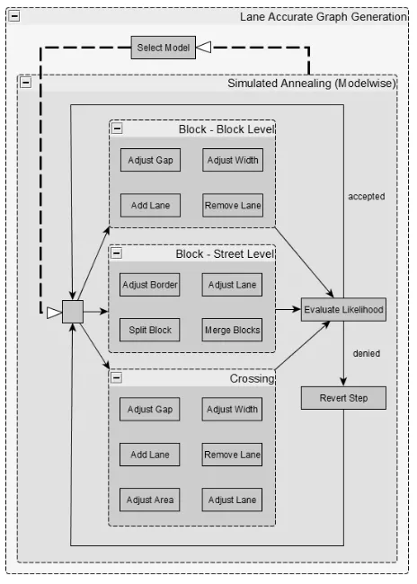
Fig. 4 gives an overview of the iterative process. It states that firstly a model (block or crossing) is selected. Secondly, an op-eration is chosen independently from the current state based on a uniform distribution and, finally, the MH step is performed by the decision on acceptance or rejection. There are three levels of operations, two of them are related to block models. Block-leveloperations affect the internal properties of a block like the number of lanes whileStreetleveloperations affect the external properties like the parametrization borders on the street. Regard-ing the probabilityzofor choosing an operation0≤zo≤1and Pz
o = 1applies. Theadd lane,remove lane,split blockand
merge blockoperations are increasing or decreasing the dimen-sion of the modelθby1while the other operations only vary the existing parameters.
The overall algorithm can be summarized into the following steps:
1. Create a road accurate network from the input trajectory data
2. Transfer the network to parameterized models and initialize all blocks and intersections
3. Each model: Iterationi
- Samplew∼Unif[0,1]
- Select an operation depending onw(Fig. 4)
- Calculate the acceptance probability according to the operation and perform a MH step
- Accept or reject the step. If the step is rejected, the operation is reverted
4. Update the cooling function
5. i←i+ 1and go to 3.
In the following, the operations are considered in detail and in terms of unification hereafter a modelξis in the context of RJM-CMC referred to as a stateθ(see Section 3.1 and 3.2).
Figure 4. Abstract procedure of the optimization. In each iteration firstly the model and secondly the operation is selected.
The operationadd lanecan add a new lane to a block on the right or left side. Thus, the state is complemented by an additional lane width. The initial lane width is sampled from a normal distribu-tion which complies with thedirective of urban traffic with public bus servicein accordance with (Baier et al., 2006) and applies to our urban scenario.
The dimension transition function in accordance to Section 3.2 is defined as
τb,add(θ, u) = (θ, u)
u∼N(3.25,0.5)
and the add lane acceptance ratio is
bb,add((ki, θi),(kj, θj)) = min{1, B}
B=zij·πj(θj)
zji·πi(θi)
·q|Jτ|i|
2πσ2 b,add
·exp(−(u−µb,add)
2
2σ2 b,add
)
In this case, the Jacobian matrix is 1. Similarly, a lane can be removed the inverse way, therefore the acceptance ratio is
bb,rem(·|·) =min{1, B−1}
whereuis replaced by the width of the removed lane.
Street level operations The operationadjust bordervaries the parametrization borders of the block on the street level. Thus, the block can be extended or shortened longitudinally. The operation adjust lanevaries the length of the direction vectors of the cubic Hermite splines representing the centerline of a block. This way
the curvature of the street course can be influenced and therefore a block can be adapted to a curve with arbitrary radius. The op-erationsplit blockcan divide a block into two individual blocks. This step generates a new block model with the same properties as the original block, thus no special acceptance ratio but a slight modification to the interpretation of the posterior distribution is needed. Normally, the evaluation of the new and the old state are compared in the MH step. However, in this case, the eval-uation of the original block is compared with the average value of the two resulting blocks. The other way around, the operation merge blockcan unite two adjacent blocks into one and the MH step deals with the average evaluation of the merged blocks on the one hand and with the evaluation of the resulting block on the other. All operations can be realized with a random walk proposal function.
Crossing operations The crossing operations are equal to the block- and streetlevel operations. Additionally,adjust areachange the parameters defining the spatial extension of the crossing. Thus, this operation changes the surface of the intersection and can be realized by a random walk proposal function.
5. RESULTS
In this section our algorithm is applied to a dataset in three dif-ferent accuracy levels, which are described in Section 5.1. In Section 5.2 the results are evaluated against a LIDAR based lane accurate network map (Section 5.1.2).
5.1 Input Data
5.1.1 Trajectory Data To assess the quality of the results of our algorithm we recorded ego trajectory data. The test vehi-cle was equipped with an Applanix POS LV1 system compris-ing a 220 channel GNSS receiver (GPS-17 component), a set of Trimble 540 AP antennas, aninertial measurement unit(IMU-42 component) and adistance measurement instrument(DMI). Ad-ditionally, we made use of the SAPOS2services, a satellite refer-ence service which can be used to increase the position accuracy. This hard- and software setting enabled us to record the dataset in three different accuracy levels. The first level comprises data recorded with the GPS system only. In the second level, these data are merged with the IMU und DMI data. Finally, the sec-ond level data are merged with post processing data from SAPOS to reach a high accuracy level. The dataset maps an inner city scenario comprising two intersections and seven roads with high traffic volume as it can be seen in Fig. 5a. Per level it consists of54trips with an overall length of about32km running at an average speed of about30km/h and is recorded in1Hz. The datasets reach an average position error of1.65 m, 1.19 mand 0.20 m(data from Applanix system) in the three accuracy levels, respectively.
5.1.2 Ground Truth Data For the evaluation, we use a high accurate LIDAR based map3which fulfills particularly high re-quirements in accuracy. The used laser scanner has a measure-ment error of about 2cm which results in combination with a differential GPS system in an absolute geo-referenced position error of10cm. The map is generated semi-automatically, with a considerable amount of human post-processing, out of the point
1POS LV 220 V5 System (http://www.applanix.com/) 2http://www.sapos.de/
3generated by http://www.3d-mapping.de/
This contribution has been peer-reviewed. The double-blind peer-review was conducted on the basis of the full paper.
(a) Trajectory input data of the scenario (b) Exemplary reconstructions
Figure 5. Raw trajectory input data of the scenario and exemplary reconstructions as quantitative results.
cloud of the laser scanner and results in an NDS4associated map with lane accurate topological and geometrical information. The map comprises the centerlines of the lanes which implies their widths and is represented as a graph which implies the connec-tivity.
5.2 Evaluation
In this subsection, the results produced by our algorithm, based on level three input data, are qualitatively evaluated. To this end, we matched the reconstructed map to the ground truth map to as-sociate the streets and crossings respectively. Based on this, on the one hand, the individual properties of the models are com-pared to state a quality measure at the model level and, on the other hand, the matching distance between the graphs is evalu-ated as a general measure. These criteria will be applied in two scales. Firstly, the mentioned measures will be applied to a sin-gle street to consider an exemplary comparison of the individual properties. Secondly, the whole scenario is taken into account to assess its overall quality. Furthermore, we applied two path-based comparison methods to evaluate the topology and geometry in a sufficient way.
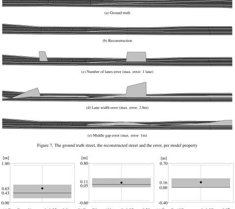
Regarding a single street from the third stage dataset of a length of about200 m, we analyzed the total error in terms of each param-eter of the model. In Fig. 7 the street model is shown in a three di-mensional context where the vertical dimension is the magnitude of the error. Fig. 7a shows the ground truth and Fig. 7b the re-constructed street. Fig. 6 presents the total matching error of the lane’s centerlines of both graphs as a boxplot5with a span from 0.03 mto0.34 m, a mean of0.2 mand a median of0.15 m. In Fig. 7c the error regarding the number of lanes can be seen. Ob-viously, in the middle of the street the corresponding block is too short which results in a missing lane error. This error is difficult to avoid since the exact position of an upcoming lane can only be es-timated from the trajectories. Overall this exemplary street model reconstructed92%of the road correctly regarding the property of lane numbers. Fig. 7d shows the difference of the lane width of the associated lanes. It is striking that in therightsection where a lane is missing the match of the lanes fails. In this case, the upcoming lane is matched to a remaining one which results in an error that is already detected (in the number of lane property). There is one more conspicuous error in the most left block which originates from a new lane in the ground truth map which is not upcoming but appearing. This characteristic cannot be derived
4Navigation Data Standard, http://www.nds-association.org/ 5Data division: bottom whisker: 0%, gray box: 25%-75%, black line
(median): 50%, black point: average value, upper whisker: 100%
from the trajectories only, thus, the error cannot be avoided. On the remaining parts of the street, the matches are correct and the error of the reconstructed lane widths is0.2 min average. Fi-nally, Fig. 7e shows the error concerning the gap between the op-posite driving directions. In this example, the gap’s shape is quite complex and can be estimated with an average error of0.4 m.
0.0 0.35 [m]
0.20 0.15
Figure 6. Matching error of the lane’s centerlines [m]. Min.:0.03 m, Median:0.15 m, Mean:0.2 m, Max.:0.34 m
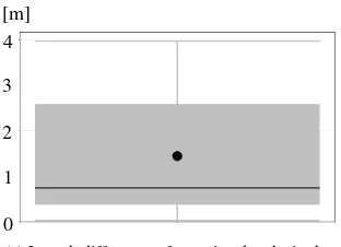
Investigating a single street, the mentioned properties can be vi-sualized as it is shown in Fig. 7. Regarding the whole scenario these properties must be quantified and therefore Fig. 8 shows the overall matching, lane width and middle gap error as boxplots. To create these result datasets, each street model is discretized in portions of1 mlength which are then evaluated. Fig. 8a states an overall matching error out of[0; 1.75] mwhich implies, that there is at least one perfect match of0 mand one worse match which is likely caused by a missing lane and thus is of the dimen-sion of half a lane width. Fig. 8b presents the overall error of the lane width estimation in the range of[−0.53; 0.75] m. Here, the errors caused by mismatches of upcoming lanes as it is occurred in Fig. 7d are filtered since these errors are already accounted for in the matching error. This criteria is evaluated in both direc-tions, which means, that a negative value implies a too narrow reconstruction of the lane and the other way around respectively. Finally, Fig. 8c shows the overall error of the middle gap estima-tion out of[−0.37; 0.68] mwhich is evaluated in both directions too. Overall, the quite low quantitative errors of the individual properties and additionally the visual comparison of Fig. 7a and 7b show the large potential of the method for ADAS applications, such as lane accurate route planning and navigation.
(a) Ground truth
(b) Reconstruction
(c) Number of lanes error (max. error: 1 lane)
(d) Lane width error (max. error: 2.8m)
(e) Middle gap error (max. error: 1m)
Figure 7. The ground truth street, the reconstructed street and the error, per model property
0.00 1.80 [m]
0.43 0.65
(a) Overall matching error [m]. Min.:0
.0 m, Median:0
.43 m, Mean:0.65 m, Max.:1.75 m -0.60
0.05 0.80 [m]
0.11
(b) Overall lane width error [m]. Min.:−0.53 m, Median:0
.05 m, Mean:0.11 m, Max.:0.75 m -0.40
0.00 0.70 [m]
0.16
(c) Overall middle gap error [m]. Min.:−0.37 m, Median:0
.0 m, Mean:0.16 m, Max.:0.68 m
Figure 8. Overall error
dH(X, Y) = max
sup
x∈X
inf
y∈Yd(x, y),ysup∈Yxinf∈Xd(x, y)
.
The result of the length comparison is shown in Fig. 9a. This is a major measure of the topological similarity of the graphs. A topological error like a missing street lane or crossing connec-tion will result in a different path, usually of different length. In comparison, geometrical errors will only have a minor impact. In Fig. 9b the Hausdorff distance of the paths can be seen which is a major measure of the geometrical similarity. Here, geometrical errors like lane widths, middle gap or position errors will result in an offset which increases the Hausdorff distance. Topologi-cal errors have an impact too, because a significant different path causes a great distance.
The presented results in Fig. 8 and Fig. 9 are generated based on the level three accuracy dataset. The corresponding results of the first dataset, comprising GPS data only, are summarized in Table 1. The evaluations of the second dataset, comprising GPS, IMU and DMI, are shown in Table 2.
Criteria Min. Median Mean Max.
Matching error 0.0 1.22 1.44 2.89
Lane width error -0.57 0.07 0.17 0.83
Middle gap error -1.17 0.0 0.34 1.96
Path length difference 0.44 3.72 4.89 13.30 Path Hausdorff distance 1.22 3.74 5.01 9.74
Table 1. Stage 1 (GPS) evaluation [m]
Criteria Min. Median Mean Max.
Matching error 0.0 1.01 1.18 2.71
Lane width error -0.49 0.07 0.16 0.74
Middle gap error -1.11 0.47 0.41 1.90
Path length difference 0.38 3.18 3.65 9.47 Path Hausdorff distance 0.83 3.53 4.65 7.97
Table 2. Stage 2 (GPS, IMU, DMI) evaluation [m]
This contribution has been peer-reviewed. The double-blind peer-review was conducted on the basis of the full paper.
4
0 1 2 3 [m]
(a) Length difference of associated paths in the reconstructed and the ground truth map [m]. Min.:0
.03 m, Median:0.74 m, Mean:1.45 m, Max.:3
.97 m
3
0 1 2 [m]
(b) Hausdorff metric of associated paths in the reconstructed and the ground truth map [m]. Min.:0
.70 m, Median:2.25 m, Mean:2.27 m, Max.:3
.62 m
Figure 9. Path-based evaluation results
Accuracy Level Median error Mean error
Stage 1 0.65% 0.85%
Stage 2 0.55% 0.63%
Stage 3 0.13% 0.25%
Table 3. Relative error of path length differences (absolute error in Table 1 & 2 and Fig. 9a)
Since the length difference error is a measure depending on the individual trajectory it can be transformed to a relative error by relating it to the trajectories length. The relative errors are shown in Table 3 which states a path length difference error of less than 1%for each stage.
Overall, our algorithm produces satisfying results regarding mea-sures of the internal properties and of the structural characteris-tics. Some more results of a crossing and a street are shown in Fig, 5b.
6. CONCLUSION AND FUTURE WORK
In this paper a new approach for the derivation of lane accu-rate maps from vehicle fleet motion data is presented. Basing on publicly available road network graphs, lane models as pa-rameterized blocks on the roads and intersections are initialized. The lane models are optimized and derived using a Reversible Jump Markov chain Monte Carlo approach to explore the param-eter space of the model in order to find the best possible fit be-tween the input data and the model. To evaluate the approach we recorded ego trajectory data of vehicles in three different ac-curacy levels with an overall average position error of1.65 m, 1.19 mand0.20 mrespectively. We applied the algorithm to the input data and compared it to a LIDAR based ground truth map by evaluating the individual properties of the models and different
path-based comparison methods. Both the qualitative and quanti-tative analysis of the results states a large potential of the method for generating data for ADAS applications out of vehicle fleet sensor data. In the future, we plan to extend the options of the block models catalogue to be able to cover individual situations. Currently, a road consists of constant street blocks and variable connection blocks which make it difficult to fit e.g. a temporar-ily narrowed lane which could be handled by a specialnarrowed street block. Additionally, the algorithm will be extended to de-rive information about the type of road markings, e.g. dashed lines from mono camera data.
References
Ahmed, M., Karagiorgou, S., Pfoser, D. and Wenk, C., 2015. A comparison and evaluation of map construction algorithms using vehicle tracking data. GeoInformatica19(3), pp. 601– 632.
Andrieu, C., De Freitas, N. and Doucet, A., 2000. Reversible jump mcmc simulated annealing for neural networks. In: Pro-ceedings of the Sixteenth conference on Uncertainty in artifi-cial intelligence, Morgan Kaufmann Publishers Inc., pp. 11– 18.
Baier, R., Eilrich, W., Haller, W., Heinz, H., Lentz, D., Lerner, M., Maier, R., Manns, F., M¨uller-Ettler, M., Nikolaus, H. et al., 2006. Richtlinien f¨ur die anlage von stadtstraßen. Forschungs-gesellschaft f¨ur Straßen-und Verkehrswesen.
Biagioni, J. and Eriksson, J., 2012. Map inference in the face of noise and disparity. In:Proceedings of the 20th International Conference on Advances in Geographic Information Systems, SIGSPATIAL ’12, ACM, New York, NY, USA, pp. 79–88.
Bruntrup, R., Edelkamp, S., Jabbar, S. and Scholz, B., 2005. In-cremental map generation with gps traces. In: Proceedings. 2005 IEEE Intelligent Transportation Systems, 2005., pp. 574– 579.
Catmull, E. and Rom, R., 1974. A class of local interpolating splines.Computer aided geometric design74, pp. 317–326. Green, P. J., 1995. Reversible jump markov chain monte carlo
computation and bayesian model determination. Biometrika 82(4), pp. 711–732.
Hastings, W. K., 1970. Monte carlo sampling methods us-ing markov chains and their applications. Biometrika57(1), pp. 97–109.
Karagiorgou, S. and Pfoser, D., 2012. On vehicle tracking data-based road network generation. In: Proceedings of the 20th International Conference on Advances in Geographic Infor-mation Systems, SIGSPATIAL ’12, ACM, pp. 89–98. Metropolis, N., Rosenbluth, A. W., Rosenbluth, M. N., Teller,
A. H. and Teller, E., 1953. Equation of state calculations by fast computing machines. The Journal of Chemical Physics 21(6), pp. 1087–1092.
Meyn, S. P. and Tweedie, R. L., 1993. Markov Chains and Stochastic Stability. Springer-Verlag.
Newson, P. and Krumm, J., 2009. Hidden Markov map matching through noise and sparseness. Proceedings of the 17th ACM SIGSPATIAL International Conference on Advances in Geo-graphic Information Systems - GIS ’09pp. 336–343.
![Figure 6. Matching error of the lane’s centerlines [m].](https://thumb-ap.123doks.com/thumbv2/123dok/3221500.1395346/6.595.342.500.319.420/figure-matching-error-lane-s-centerlines-m.webp)