www.elsevier.comrlocatereconbase
Estimation of tail-related risk measures for
heteroscedastic financial time series: an extreme
value approach
Alexander J. McNeil
a,), Rudiger Frey
b,1¨
a
Department of Mathematics, Swiss Federal Institute of Technology, ETH Zentrum, CH-8092 Zurich, Switzerland
b
Swiss Banking Institute, UniÕersity of Zurich, Plattenstrasse 14, CH-8032 Zurich, Switzerland
Abstract
Ž .
We propose a method for estimating Value at Risk VaR and related risk measures describing the tail of the conditional distribution of a heteroscedastic financial return series. Our approach combines pseudo-maximum-likelihood fitting of GARCH models to estimate
Ž .
the current volatility and extreme value theory EVT for estimating the tail of the innovation distribution of the GARCH model. We use our method to estimate conditional
Ž . Ž
quantiles VaR and conditional expected shortfalls the expected size of a return exceeding .
VaR , this being an alternative measure of tail risk with better theoretical properties than the quantile. Using backtesting of historical daily return series we show that our procedure gives better 1-day estimates than methods which ignore the heavy tails of the innovations or the stochastic nature of the volatility. With the help of our fitted models we adopt a Monte Carlo approach to estimating the conditional quantiles of returns over multiple-day horizons and find that this outperforms the simple square-root-of-time scaling method. q2000 Elsevier Science B.V. All rights reserved.
JEL classification: C.22; G.10; G.21
Keywords: Risk measures; Value at risk; Financial time series; GARCH models; Extreme value theory; Backtesting
)
Corresponding author. Tel.:q41-1-632-61-62; fax:q41-1-632-15-23.
Ž . Ž .
E-mail addresses: [email protected] A.J. McNeil , [email protected] R. Frey .
1
Tel.:q41-1-634-29-57; fax:q41-1-634-49-03.
0927-5398r00r$ - see front matterq2000 Elsevier Science B.V. All rights reserved.
Ž .
1. Introduction
The large increase in the number of traded assets in the portfolio of most Ž
financial institutions has made the measurement of market risk the risk that a financial institution incurs losses on its trading book due to adverse market
.
movements a primary concern for regulators and for internal risk control. In particular, banks are now required to hold a certain amount of capital as a cushion against adverse market movements. According to the Capital Adequacy Directive
Ž . Ž .
by the Bank of International Settlement BIS in Basle, Basle Comittee, 1996 the risk capital of a bank must be sufficient to cover losses on the bank’s trading portfolio over a 10-day holding period in 99% of occasions. This value is usually
Ž .
referred to as Value at Risk VaR . Of course, holding period and confidence level may vary according to application; for purposes of internal risk control most financial firms also use a holding period of one day and a confidence level of 95%. From a mathematical viewpoint VaR is simply a quantile of the
Profit-and-Ž .
Loss P & L distribution of a given portfolio over a prescribed holding period. Alternative measures of market risk have been proposed in the literature. In two
Ž .
recent papers, Artzner et al. 1997, 1999 show that VaR has various theoretical deficiencies as a measure of market risk; they propose the use of the so-called
expected shortfall or tail conditional expectation instead. The expected shortfall
measures the expected loss given that the loss L exceeds VaR; in mathematical
w < x
terms it is given by E L L)VaR . From a statistical viewpoint the main challenge in implementing one of these risk-measures is to come up with a good estimate for the tails of the underlying P & L distribution; given such an estimate both VaR and expected shortfall are fairly easy to compute.
In this paper we are concerned with tail estimation for financial return series. Our basic idealisation is that returns follow a stationary time series model with stochastic volatility structure. There is strong empirical support for stochastic
Ž .
volatility in financial time series; see for instance Pagan 1996 . The presence of stochastic volatility implies that returns are not necessarily independent over time. Hence, with such models there are two types of return distribution to be consid-ered — the conditional return distribution where the conditioning is on the current volatility and the marginal or stationary distribution of the process.
Both distributions are of relevance to risk managers. A risk-manager who wants to measure the market risk of a given portfolio is mainly concerned with the possible extent of a loss caused by an adverse market movement over the next day Žor next few days given the current volatility background. His main interest is in. the tails of the conditional return distribution, which are also the focus of the present paper. The estimation of unconditional tails provides different, but comple-mentary information about risk. Here we take the long-term view and attempt to
Ž assign a magnitude to a specified rare adverse event, such as a 5-year loss the size
.
information may be of interest to the risk manager who wishes to perform a scenario analysis and get a feeling for the scale of worst case or stress losses.
In a referee’s report the concern was raised that the use of conditional return distributions for market risk measurement might lead to capital requirements that fluctuate wildly over time and are therefore difficult to implement. Our answer to this important point is threefold. First, while it is admittedly impossible for a financial institution to rapidly adjust its capital base to changing market condi-tions, the firm might very well be able to adjust the size of its exposure instead. Moreover, besides providing a basis for the determination of risk capital, measures of market risk are also employed to give the management of a financial firm a better understanding of the riskiness of its portfolio, or parts thereof. We are convinced that the riskiness of a portfolio does indeed vary with the general level of market volatility, so that the current volatility background should be reflected in the risk-numbers reported to management. Finally, we think that the economic problem of defining an appropriate risk-measure for setting capital-adequacy standards should be separated from the statistical problem of estimating a given measure of market risk, which is the focus of the present paper.
Schematically the existing approaches for estimating the P & L distribution of a portfolio of securities can be divided into three groups: the non-parametric
Ž .
historical simulation HS method; fully parametric methods based on an econo-metric model for volatility dynamics and the assumption of conditional normality Že.g. J.P. Morgan’s Riskmetrics and most models from the ARCHrGARCH
. Ž .
family ; and finally methods based on extreme value theory EVT .
In the HS-approach the estimated P & L distribution of a portfolio is simply given by the empirical distribution of past gains and losses on this portfolio. The method is therefore easy to implement and avoids Aad-hoc-assumptionsB on the form of the P & L distribution. However, the method suffers from some serious drawbacks. Extreme quantiles are notoriously difficult to estimate, as extrapolation beyond past observations is impossible and extreme quantile estimates within sample tend to be very inefficient — the estimator is subject to a high variance. Furthermore, if we seek to mitigate these problems by considering long samples the method is unable to distinguish between periods of high and low volatility.
Econometric models of volatility dynamics that assume conditional normality, such as GARCH-models, do yield VaR estimates which reflect the current volatility background. The main weakness of this approach is that the assumption of conditional normality does not seem to hold for real data. As shown, for
Ž .
instance, in Danielsson and de Vries 1997b , models based on conditional normality are therefore not well suited to estimating large quantiles of the P & L-distribution.2
2
Note that the marginal distribution of a GARCH-model with normally distributed errors is usually fat-tailed as it is a mixture of normal distributions. However, this matters only for quantile estimation
Ž .
The estimation of return distributions of financial time series via EVT is a Ž
topical issue which has given rise to some recent work Embrechts et al., 1998, 1999; Longin, 1997a,b; McNeil, 1997, 1998; Danielsson and de Vries, 1997b,
.
1997c; Danielsson et al., 1998 . In all these papers the focus is on estimating the
Ž . Ž .
unconditional stationary distribution of asset returns. Longin 1997b and McNeil Ž1998 use estimation techniques based on limit theorems for block maxima.. Longin ignores the stochastic volatility exhibited by most financial return series and simply applies estimators for the iid-case. McNeil uses a similar approach but shows how to correct for the clustering of extremal events caused by stochastic
Ž .
volatility. Danielsson and de Vries 1997a,b use a semiparametric approach based
Ž .
on the Hill-estimator of the tail index. Embrechts et al. 1999 advocate the use of a parametric estimation technique which is based on a limit result for the excess-distribution over high thresholds. This approach will be adopted in this paper and explained in detail in Section 2.2.
EVT-based methods have two features which make them attractive for tail estimation: they are based on a sound statistical theory; they offer a parametric form for the tail of a distribution. Hence, these methods allow for some extrapola-tion beyond the range of the data, even if care is required at this point. However, none of the previous EVT-based methods for quantile estimation yields VaR-estimates which reflect the current volatility background. Given the conditional heteroscedasticity of most financial data, which is well documented by the considerable success of the models from the ARCHrGARCH family, we believe this to be a major drawback of any kind of VaR-estimator.
In order to overcome the drawbacks of each of the above methods we combine ideas from all three approaches. We use GARCH-modelling and pseudo-maxi-mum-likelihood estimation to obtain estimates of the conditional volatility. Statis-tical tests and exploratory data analysis confirm that the error terms or residuals do form, at least approximately, iid series that exhibit heavy tails. We use historical
Ž .
simulation for the central part of the distribution and threshold methods from
Ž .
EVT for the tails to estimate the distribution of the residuals. The application of
Ž .
these methods is facilitated by the approximate independence over time of the residuals. An estimate of the conditional return distribution is now easily con-structed from the estimated distribution of the residuals and estimates of the conditional mean and volatility. This approach reflects two stylized facts exhibited by most financial return series, namely stochastic volatility and the fat-tailedness of conditional return distributions over short time horizons.
Ž .
from EVT will give better estimates of the tails of the residuals. During the revision of this paper we also learned that the central idea of our approach — the application of EVT to model residuals — has been independently proposed by
Ž .
Diebold et al. 1999 .
We test our approach on various return series. Backtesting shows that it yields better estimates of VaR and expected shortfall than unconditional EVT or GARCH-modelling with normally distributed error terms. In particular, our
analy-Ž .
sis contradicts Danielsson and de Vries 1997c , who state thatAan unconditional approach is better suited for VaR estimation than conditional volatility forecastsB
Žpage 3 of their paper . On the other hand, we see that models with a normally. distributed conditional return distribution yield very bad estimates of the expected shortfall, so that there is a real need for working with leptokurtic error distribu-tions. We also study quantile estimation over longer time-horizons using
simula-Ž tion. This is of interest if we want to obtain an estimate of the 10-day VaR as
.
required by the BIS-rule from a model fitted to daily data.
2. Methods
Ž .
Let X , tt gZ be a strictly stationary time series representing daily observa-tions of the negative log return on a financial asset price.3 We assume that the
dynamics of X are given by
XtsmtqstZ ,t
Ž .
1Ž
where the innovations Z are a strict white noise processt i.e. independent, .
identically distributed with zero mean, unit variance and marginal distribution Ž .
function F z . We assume that m and s are measurable with respect to GG ,
Z t t t -1
the information about the return process available up to time ty1.
Ž . Ž .
Let FX x denote the marginal distribution of Xt and, for a horizon hgN, Ž .
let FXt q. . .qX <GG x denote the predictive distribution of the return over the
q1 tqh t
next h days, given knowledge of returns up to and including day t. We are interested in estimating quantiles in the tails of these distributions. For 0-q-1, an unconditional quantile is a quantile of the marginal distribution denoted by
xqsinf x
gR: FXŽ .
x Gq ,4
3
and a conditional quantile is a quantile of the predictive distribution for the return over the next h days denoted by
xqt
Ž .
h sinf x gR: FXt q. . .qX <GGŽ .
x Gq .4
q1 tqh t
We also consider an alternative measure of risk for the tail of a distribution known as the expected shortfall. The unconditional expected shortfall is defined to be
<
SqsE X X)xq ,
and the conditional expected shortfall to be
h h
t < t
S
Ž .
h sEÝ
XÝ
X )xŽ .
h ,GG .q tqj tqj q t
js1 js1
We are principally interested in quantiles and expected shortfalls for the 1-step predictive distribution, which we denote respectively by xqt and Sqt. Since
<
where zq is the upper qth quantile of the marginal distribution of Z which byt assumption does not depend on t.
To implement an estimation procedure for these measures we must choose a Ž .
specific process in the class 1 , i.e. a particular model for the dynamics of the conditional mean and volatility. Many different models for volatility dynamics have been proposed in the econometric literature including models from the
Ž . Ž
ARCHrGARCH family Bollerslev et al., 1992 , HARCH processes Muller et
¨
. Ž .
al., 1997 and stochastic volatility models Shephard, 1996 . In this paper, we use Ž .
the parsimonious but effective GARCH 1,1 process for the volatility and an Ž .
AR 1 model for the dynamics of the conditional mean; the approach we propose extends easily to more complex models.
In estimating xqt with GARCH-type models it is commonly assumed that the innovation distribution is standard normal so that a quantile of the innovation
y1Ž . Ž .
distribution is simply zqsF q , where F z is the standard normal d.f. A
GARCH-type model with normal innovations can be fitted by maximum
likeli-Ž .
hood ML and mtq1 and stq1 can be estimated using standard 1-step forecasts,
t Ž .
so that an estimate of x is easily constructed using 3 . This is close in spirit toq
Ž .
conditional quantile for q)0.95; the distribution of the innovations seems generally to be heavier-tailed or more leptokurtic than the normal.
Another standard approach is to assume that the innovations have a leptokurtic
Ž .
distribution such as Student’s t-distribution scaled to have variance 1 . Suppose
(
Zs
Ž
ny2.
rnT where T has a t-distribution on n)2 degrees of freedom withy1
Ž .
(
Ž .d.f. F t . Then zT qs
Ž
ny2.
rnFT q . GARCH-type models witht-innova-tions can also be fitted with maximum likelihood and the additional parametern
can be estimated. We will see in Section 2.2 that this method can be viewed as a special case of our approach; it yields quite satisfactory results as long as the
Ž .
positive and the negative tail of the return distribution are roughly equal. The method proposed in this paper makes minimal assumptions about the underlying innovation distribution and concentrates on modelling its tail using EVT. We use a two-stage approach which can be summarised as follows.
Ž . 1. Fit a GARCH-type model to the return data making no assumption about F zZ
Ž .
and using a pseudo-maximum-likelihood approach PML . Estimate mtq1 and
stq1 using the fitted model and calculate the implied model residuals. 2. Consider the residuals to be a realisation of a strict white noise process and use
Ž . Ž .
extreme value theory EVT to model the tail of F z . Use this EVT model toZ estimate z for qq )0.95.
We go into these stages in more detail in the next sections and illustrate them by means of an example using daily negative log returns on the Standard and Poors index.
2.1. Estimatingstq1 andmtq1 using PML
For predictive purposes we fix a constant memory n so that at the end of day t
Ž .
our data consist of the last n negative log returns xtynq1, . . . , xty1, x . Wet
Ž . Ž .
consider these to be a realisation from a AR 1 –GARCH 1,1 process. Hence, the conditional variance of the mean-adjusted series etsXtymt is given by
s2
This model is a special case of the general first order stochastic volatility process
Ž . Ž .
considered by Duan 1997 , who uses a result by Brandt 1986 to give conditions Ž .
for strict stationarity. The mean-adjusted series et is strictly stationary if
2
E log
Ž
bqa1Zty1.
-0.Ž .
6Ž .
By using Jensen’s inequality and the convexity of ylog x it is seen that a Ž .
sufficient condition for Eq. 6 is that bqa1-1, which moreover ensures that Ž .
This model is fitted using the PML method. This means that the likelihood for a Ž .
GARCH 1,1 model with normal innovations is maximized to obtain parameter
ˆ
Žˆ
ˆ
.Testimates us f, a
ˆ
0, aˆ
1, b . While this amounts to fitting a model using a distributional assumption we do not necessarily believe, the PML method delivers reasonable parameter estimates. In fact, it can be shown that the PML method yields a consistent and asymptotically normal estimator; see for instance Chapter 4Ž .
of Gourieroux 1997 .
´
Ž
Estimates of the conditional mean and standard deviation series m
ˆ
tynq1, . . . ,. Ž . Ž . Ž .
m
ˆ
t and sˆ
tynq1, . . . , sˆ
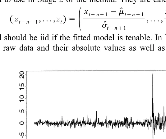
t can be calculated recursively from Eqs. 4 and 5 after substitution of sensible starting values. In Fig. 1 we show an arbitrary thousand day excerpt from our dataset containing the stock market crash of October 1987; the estimated conditional standard deviation derived from the GARCH fit is shown below the series.Residuals are calculated both to check the adequacy of the GARCH modelling and to use in Stage 2 of the method. They are calculated as
xtynq1ym
ˆ
tynq1 xtymˆ
t z , . . . , z s , . . . , ,Ž
tynq1 t.
ž
s s/
ˆ
tynq1ˆ
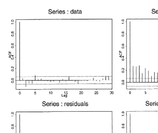
tand should be iid if the fitted model is tenable. In Fig. 2 we plot correlograms for the raw data and their absolute values as well as for the residuals and absolute
Fig. 1. 1000 day excerpt from series of negative log returns on Standard and Poors index containing crash of 1987; lower plot shows estimate of the conditional standard deviation derived from PML
Ž . Ž .
Fig. 2. Correlograms for the raw data and their absolute values as well as for the residuals and absolute residuals. While the raw data are clearly not iid, this assumption may be tenable for the residuals.
residuals. While the raw data are clearly not iid, this assumption may be tenable for the residuals.4
If we are satisfied with the fitted model, we end stage 1 by calculating estimates of the conditional mean and variance for day tq1, which are the obvious 1-step forecasts
ˆ
m
ˆ
tq1sfx ,t$ $
2 2
ˆ
2s
ˆ
tq1sa0qa e1 tˆ
qbsˆ
t ,wheree
ˆ
tsxtymˆ
t.4
2.2. Estimating z using EVTq
We begin stage 2 by forming a QQ-Plot of the residuals against the normal distribution to confirm that an assumption of conditional normality is unrealistic, and that the innovation process has fat tails or is leptokurtic — see Fig. 3.
We then fix a high threshold u and we assume that excess residuals over this
Ž .
threshold have a generalized Pareto distribution GPD with d.f.
y1rj
1y
Ž
1qjyrb.
ifj/0,Gj,b
Ž .
y s½
1yexp
Ž
yyrb.
ifjs0,where b)0, and the support is yG0 when jG0 and 0FyFybrj when
j-0.
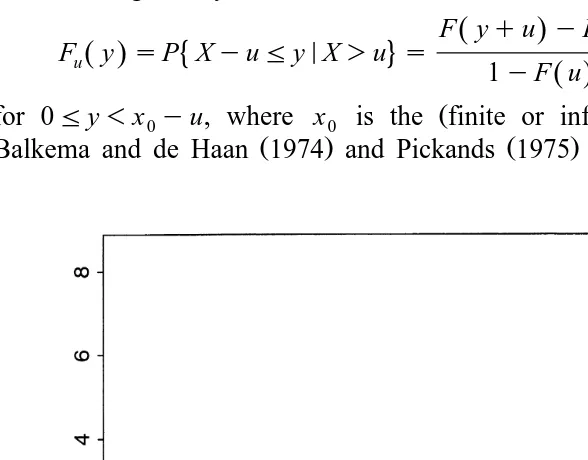
This particular distributional choice is motivated by a limit result in EVT. Consider a general d.f. F and the corresponding excess distribution above the threshold u given by
F y
Ž
qu.
yF uŽ .
4
Fu
Ž .
y sP XyuFyNX)u s , 1yF uŽ .
Ž .
for 0Fy-x0yu, where x0 is the finite or infinite right endpoint of F.
Ž . Ž .
Balkema and de Haan 1974 and Pickands 1975 showed for a large class of
Ž . distributions F that it is possible to find a positive measurable function b u such
that
For more details consult Theorem 3.4.13 on page 165 of Embrechts et al. 1997 . In the class of distributions for which this result holds are essentially all the common continuous distributions of statistics5, and these may be further
subdi-vided into three groups according to the value of the parameterj in the limiting GPD approximation to the excess distribution. The case j)0 corresponds to heavy-tailed distributions whose tails decay like power functions, such as the Pareto, Student’s t, Cauchy, Burr, loggamma and Frechet distributions. The case
´
js0 corresponds to distributions like the normal, exponential, gamma and lognormal, whose tails essentially decay exponentially. The final group ofdistribu-Ž .
tions are short-tailed distributions j-0 with a finite right endpoint, such as the uniform and beta distributions.
We assume the tail of the underlying distribution begins at the threshold u. From our sample of n points a random number NsNu)0 will exceed this threshold. If we assume that the N excesses over the threshold are iid with exact
Ž .
GPD distribution, Smith 1987 has shown that maximum likelihood estimates
ˆ
ˆ
ˆ
ˆ
jsjN and bsbN of the GPD parameters j andb are consistent and asymptoti-cally normal as N™`, provided j)y1r2. Under the weaker assumption that
Ž .
the excesses are iid from F y which is only approximately GPD he also obtainsu
ˆ
ˆ
asymptotic normality results forj andb. By letting usun™x and N0 sNu™`
as n™` he shows essentially that the procedure is asymptotically unbiased provided that u™x sufficiently fast. The necessary speed depends on the rate of0
Ž .
convergence in Eq. 7 . In practical terms, this means that our best GPD estimator of the excess distribution is obtained by trading bias off against variance. We
Ž .
choose u high to reduce the chance of bias while keeping N large i.e. u low to
Ž .
control the variance of the parameter estimates. The choice of u or N is the most important implementation issue in EVT and we discuss this issue in the context of finite samples from typical return distributions in Section 2.3.
Consider now the following equality for points x)u in the tail of F
1yF x
Ž .
sŽ
1yF uŽ .
.
Ž
1yFuŽ
xyu.
.
.Ž .
8 Ž .If we estimate the first term on the right hand side of Eq. 8 using the random proportion of the data in the tail Nrn, and if we estimate the second term by
5
approximating the excess distribution with a generalized Pareto distribution fitted by maximum likelihood, we get the tail estimator
ˆ
for x)u. Smith 1987 also investigates the asymptotic relative error of this
estimator and gets a result of the form
$ quires that u™x sufficiently fast.0
In practice we will actually modify the procedure slightly and fix the number of data in the tail to be Nsk where k<n. This effectively gives us a random
Ž .
threshold at the kq1 th order statistic. Let zŽ1.GzŽ2.G. . .GzŽn. represent the ordered residuals. The generalized Pareto distribution with parameters j and b is
Ž .
fitted to the data zŽ1.yzŽkq1., . . . , zŽk.yzŽkq1. , the excess amounts over the threshold for all residuals exceeding the threshold. The form of the tail estimator
Ž .
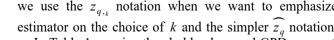
we use the zq ,k notation when we want to emphasize the dependence of the$ estimator on the choice of k and the simpler z notation otherwise.q
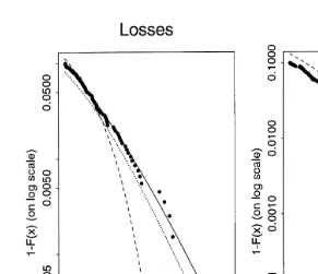
In Table 1 we give threshold values and GPD parameter estimates for both tails of the innovation distribution of the test data in the case that ns1000 and
ks100; we discuss this choice of k in Section 2.3. In Fig. 4 we show the
Table 1
Threshold values and maximum likelihood GPD parameter estimates used in the construction of tail estimators for both tails of the innovation distribution of the test data. Note that ks100 in both cases.
Ž .
Standard errors s.e.s are calculated using a standard likelihood approach based on the observed Fisher information matrix
ˆ ˆ
Tail zŽkq1. j s.e. b s.e.
Ž . Ž .
Losses 1.215 0.224 0.122 0.568 0.089
Ž . Ž .
Fig. 4. GPD tail estimates for both tails of the innovations distribution. The points show the empirical distribution of the residuals and the solid lines represent the tail estimates. Also shown are the d.f. of
Ž . Ž .
the standard normal distribution dashed and the d.f. of the t-distribution dotted with degrees of
Ž . Ž .
freedom as estimated in an AR 1 –GARCH 1,1 model with t-innovations.
Ž Ž ..
corresponding tail estimators Eq. 9 . We are principally interested in the left picture marked Losses which corresponds to large positive residuals. The solid lines in both pictures correspond to the GPD tail estimates and can be seen to model the residuals well. Also shown is a dashed line which corresponds to the standard normal distribution and a dotted line which corresponds to the estimated
Ž .
conditional t distribution scaled to have variance 1 in a GARCH model with
t-innovations. The normal distribution clearly underestimates the extent of large
losses and also of the largest gains, which we would already expect from the QQ-plot. The t-distribution, on the other hand, underestimates the losses and overestimates the gains. This illustrates the drawbacks of using a symmetric distribution with data which are asymmetric in the tails.
With more symmetric data the conditional t-distribution often works quite well and it can, in fact, be viewed as a special case of our method. As already mentioned, it is an example of a heavy-tailed distribution, i.e. a distribution whose
Ž .
limiting excess distribution is GPD with j)0. Gnedenko 1943 characterized all such distributions as having tails of the form
Ž .
where L x is a slowly varying function and j is the positive parameter of the limiting GPD. 1rj is often referred to as the tail index of F. For the t-distribu-tion with n degrees of freedom the tail can be shown to satisfy
nŽny2.r2
yn
1yF x
Ž .
; x ,Ž
12.
B 1
Ž
r2,nr2.
Ž .
where B a, b denotes the beta function, so that this provides a very simple example of a symmetric distribution in this class, and the value of j in the
Ž
limiting GPD is the reciprocal of the degrees of freedom see McNeil and Saladin Ž1997 ...
Fitting a GARCH model with t innovations can be thought of as estimating the
j in our GPD tail estimator by simpler means. Inspection of the form of the likelihood of the t-distribution shows that the estimate of n will be sensitive mainly to large observations so that it is not surprising that the method gives a reasonable fit in the tails although all data are used in the estimation. Our method has, however, the advantage that we have an explicit model for each tail. We estimate two parameters in each case, which gives a better fit in general.
Ž Ž ..
We also use the GPD tail estimator Eq. 9 to estimate the right tail of the Ž .
negative return distribution FX x by applying it directly to the raw return data xtynq1, . . . , x ; in this way we calculate an unconditional quantile estimate xt
ˆ
qusing unconditional EVT. We investigate whether this approach also provides reasonable estimates of xtq. It should however be noted that the assumption of independent excesses over threshold is much less satisfactory for the raw return data. The asymptotics of the GPD-based tail estimator are therefore much more poorly understood if applied directly to the raw return data.
Even if the procedure can be shown to be asymmptotically justified, in practice it is likely to give much more unstable results when applied to non-iid, finite
Ž . Ž
sample data. Embrechts et al. 1997 provide a related example see Fig. 5.5.4. on
. Ž .
page 270 ; they construct a first order autoregressive AR 1 process driven by a symmetric, heavy-tailed, iid noise, so that both noise distribution and marginal distribution of the process have the same tail index. They apply the Hill estimator Žan alternative EVT procedure described in Section 2.3 to simulated data from the.
Ž .
process and also to residuals obtained after fitting an AR 1 model to the raw data and find estimates of the tail index to be much more accurate and stable for the residuals, although the Hill estimator is theoretically consistent in both cases. This example supports the idea that pre-whitening of data through fitting of a dynamic model may be a sensible prelude to EVT analysis in practice.
2.3. Simulation study of threshold choice
Ž .
tail estimation with the approach based on the Hill estimator and the approach
Ž .
based on the empirical distribution function historical simulation .
Ž .
The Hill estimator Hill, 1975 is designed for data from heavy-tailed
distribu-Ž Ž ..
tions admitting the representation Eq. 11 with j)0. The estimator for j,
Ž .
based on the k exceedances of the kq1 th order statistic, is
k
ŽH. ŽH. y1
ˆ
ˆ
j sjk sk
Ý
log zŽj.ylog zŽkq1.,js1
and an associated quantile estimator is
ŽH.
see Danielsson and de Vries 1997b for details. The properties of these estimators have been extensively investigated in the EVT literature; in particular, a number of
Ž recent papers show consistency of the Hill estimator for dependent data Resnick
.
and Starica, 1995, 1996 and develop bootstrap methods for optimal choice of the
ˇ
ˇ
Ž .
threshold zŽkq1. Danielsson and de Vries, 1997a .
In the simulation study we generate samples of size ns1000 from Student’s
t-distribution which, as we have observed, provides a rough approximation to the
observed distribution of model residuals. The size of sample corresponds to the Ž .
window length we use in applications of the two-step method. From 12 we know the tail index of the t-distribution and quantiles are easily calculated. We calculate$
ˆ
Žjk and zq ,k the maximum-likelihood and GPD-based estimators of$ j and zq
ŽH. ŽH.
ˆ
.
based on k threshold exceedances as well as jk and zq ,k for various values of k; for the quantile estimates we restrict our attention to values of k such that
Ž .
k)1000 1yq , so that the target quantile is beyond the threshold. Of interest are
Ž .
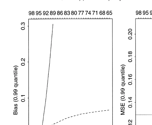
the mean squared errors MSEs and biases of these estimators, and the depen-dence of these errors on the choice of k. For each estimator we estimate MSE and bias using Monte Carlo estimates based on 1000 independent samples. For$
Ž .
where zq ,k represents the quantile estimate obtained from the jth sample. Ž Although the Hill estimator is generally the most efficient estimator of j it
.
gives the lowest MSE for sensibly chosen k it does not provide the most efficient nor the most stable quantile estimator. Our simulations suggest that the GPD method should be preferred for estimating high quantiles.
Ž .
Fig. 5. Estimated bias and MSE mean squared error against k for various estimators of the 0.99 quantile of a t distribution withns4 degrees of freedom based on an iid sample of 1000 points. Solid line is Hill estimator; dashed line is estimator based on GPD approach; dotted line is the empirical
Ž .
quantile estimator i.e. the historical simulation approach . The alternative x-axis labels above the graphs give the threshold corresponding to k expressed as a sample percentile.
estimator is marked with a dashed line and the empirical HS-estimate zŽ11. of the quantile is marked by a dotted line.
The Hill method has a negative bias for low values of k that becomes positive and then grows rapidly with k; the GPD estimator has a positive bias that grows much more slowly; the empirical estimate has a negative bias. The MSE reveals more about the relative merits of the methods: the GPD estimator attains its lowest value corresponding to a k value of about 100 but, more importantly, the MSE is very robust to the choice of k because of the slow growth of the bias. The Hill method performs well for kF70 but then deteriorates rapidly. The HS method is obviously less efficient than the two EVT methods, which shows that EVT does indeed give more precise estimates of the 99th percentile based on samples of size 1000 from the t-distribution.
because the efficient range for k is smaller; it is important that the bias be kept under control by choosing a low k.
In this paper we only show results for the t-distribution with four degrees of freedom, but further simulations suggest that the same qualitative conclusions hold for other values of n and other heavy-tailed distributions. For estimating more distant quantiles we observe that the GPD method appears to be more efficient than the Hill method and maintains its relative stability with respect to choice of k. The greater complexity of the GPD quantile estimator, which involves a second
ˆ
ˆ
y1estimated scale parameterb as well as the tail index estimatorj , seems to lead to better finite sample performance.
2.4. Summary: adÕantages of the GPD approach
We favour the GPD approach to tail estimation in this paper for a variety of reasons that we list below.
v In finite samples of the order of 1000 points from typical return distributions
Ž
EVT quantile estimators whether maximum-likelihood and GPD-based or Hill-.
based are more efficient than the historical simulation method.
v The GPD-based quantile estimator is more stable in terms of mean squaredŽ
.
error with respect to choice of k than the Hill quantile estimator. In the present application a k value of 100 seems reasonable, but we could equally choose to use
k values of 80 or 150.
vFor high quantiles with qG0.99 the GPD method is at least as efficient as the
Hill method.
v The GPD method allows effective estimates of expected shortfall to be
constructed as will be described in Section 4.
vThe GPD method is applicable to light-tailed dataŽjs0 or even short-tailed.
Ž .
data j-0 , whereas the Hill method is designed specifically for the heavy-tailed
Ž .
case j)0 . There are periods when the conditional distribution of financial returns appears light-tailed rather than heavy-tailed.
3. Backtesting
We backtest the method on five historical series of log returns: the Standard and Poors index from January 1960 to June 1993, the DAX index from January 1973 to July 1996, the BMW share price over the same period, the US dollar British pound exchange rate from January 1980 to May 1996 and the price of gold from January 1980 to December 1997.
To backtest the method on a historical series x , . . . x , where m1 m 4n, we
t 4
somewhat less than the last four years of data for each prediction. In a long backtest it is less feasible to examine the fitted model carefully every day and to choose a new value of k for the tail estimator each time; for this reason we always set ks100 in these backtests, a choice that is supported by the simulation study of the previous section. This means effectively that the 90th percentile of the innovation distribution is estimated by historical simulation, but that higher percentiles are estimated using the GPD tail estimator. On each day tgT we fit a
Ž . Ž .
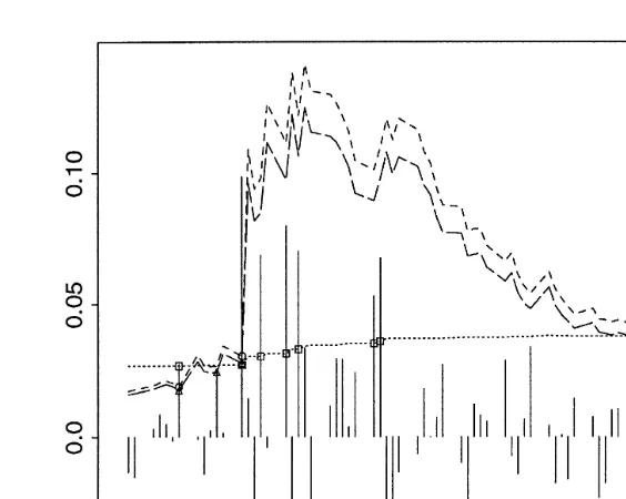
new AR 1 –GARCH 1,1 model and determine a new GPD tail estimate. Fig. 6 shows part of the backtest for the DAX index. We have plotted the negative log returns for a 3-year period commencing on the first of October 1987;
superim-t Ž .
posed on this plot is the EVT conditional quantile estimate x
ˆ
0.99 dashed line andŽ .
the EVT unconditional quantile estimate x
ˆ
0.99 dotted line .t 4
We compare x
ˆ
q with xtq1 for qg 0.95,0.99,0.995 . A violation is said to occur whenever x )xˆ
t. The violations corresponding to the backtest in Fig. 6tq1 q
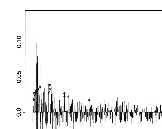
are shown in Fig. 7. We use different plotting symbols to show violations of the conditional EVT, conditional normal and unconditional EVT quantile estimates. In Fig. 8 the portion of Fig. 7 relating to the crash of October 1987 has been enlarged.
Fig. 6. Three years of the DAX backtest beginning in October 1987 and showing the EVT conditional
t Ž . Ž .
Fig. 7. Violations of xt and x corresponding to the backtest in Fig. 6. Triangles, circles and
ˆ0.99 ˆ0.99
squares denote violations of the conditional normal, conditional EVT and unconditional EVT estimates respectively. The conditional normal estimate like the conditional EVT estimate responds to changing volatility but tends to be violated rather more often, because it does not take into account the leptokurtosis of the residuals. The unconditional EVT estimate cannot respond quickly to changing volatility and tends to be violated several times in a row in stress periods.
It is possible to develop a binomial test of the success of these quantile estimation methods based on the number of violations. If we assume the dynamics
Ž .
described in Eq. 1 , the indicator for a violation at time tgT is Bernoulli
I :t s1X )xt4s1Z )z 4;Be 1
Ž
yq ..
tq1 q tq1 q
Moreover, I and I are independent for t, st s gT and t/s, since Ztq1 and Zsq1
are independent. Therefore,
I;B card T ,1
Ž
Ž .
yq ,.
Ý
t tgTi.e. the total number of violations is binomially distributed under the model. Under the null hypothesis that a method correctly estimates the conditional quantiles, the empirical version of this statistic St 1 t is from the
gT xtq1)xˆq4
Ž Ž . .
binomial distribution B card T ,1yq . We perform a two-sided binomial test of
Fig. 8. Enlarged section of Fig. 7 corresponding to the crash of 1987. Triangles, circles and squares denote violations of the conditional normal, conditional EVT and unconditional EVT estimates respectively. The dotted line shows the path of the unconditional EVT estimate, the dashed line shows the path of the conditional EVT estimate and the long dashed line shows the conditional normal estimate.
estimation error and gives too few or too many violations.6 The corresponding
binomial probabilities are given in Table 2 alongside the numbers of violations for each method. A p-value less than or equal to 0.05 will be interpreted as evidence against the null hypothesis.
In 11 out of 15 cases our approach is closest to the mark. On two occasions GARCH with conditional t innovations is best and on one occasion GARCH with conditional normal innovations is best. In one further case our approach and the
Ž conditional t approach are joint best. On no occasion does our approach fail lead
.
to rejection of the null hypothesis , whereas the conditional normal approach fails 11 times; unconditional EVT fails three times. Figs. 7 and 8 give some idea of how the latter two methods fail. The conditional normal estimate of xt like the
0.99
conditional EVT estimate responds to changing volatility but tends to be violated rather more often, because it does not take into account the leptokurtosis of the
6 Ž .
Table 2
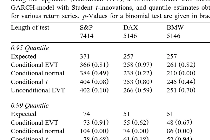
Backtesting Results: Theoretically expected number of violations and number of violations obtained
Ž .
using our approach conditional EVT , a GARCH-model with normally distributed innovations, a GARCH-model with Student t-innovations, and quantile estimates obtained from unconditional EVT for various return series. p-Values for a binomial test are given in brackets
Length of test S&P DAX BMW $r£ Gold
7414 5146 5146 3274 3413
0.95 Quantile
Expected 371 257 257 164 171
Ž . Ž . Ž . Ž . Ž .
Conditional EVT 366 0.81 258 0.97 261 0.82 151 0.32 155 0.22
Ž . Ž . Ž . Ž . Ž .
Conditional normal 384 0.49 238 0.22 210 0.00 169 0.69 122 0.00
Ž . Ž . Ž . Ž . Ž .
Conditional t 404 0.08 253 0.80 245 0.44 186 0.08 168 0.84
Ž . Ž . Ž . Ž . Ž .
Unconditional EVT 402 0.10 266 0.59 251 0.70 156 0.55 131 0.00 0.99 Quantile
Expected 74 51 51 33 34
Ž . Ž . Ž . Ž . Ž .
Conditional EVT 73 0.91 55 0.62 48 0.67 35 0.72 25 0.12
Ž . Ž . Ž . Ž . Ž .
Conditional normal 104 0.00 74 0.00 86 0.00 56 0.00 43 0.14
Ž . Ž . Ž . Ž . Ž .
Conditional t 78 0.68 61 0.18 52 0.94 40 0.22 29 0.39
Ž . Ž . Ž . Ž . Ž .
Unconditional EVT 86 0.18 59 0.29 55 0.62 35 0.72 25 0.12
0.995 Quantile
Expected 37 26 26 16 17
Ž . Ž . Ž . Ž . Ž .
Conditional EVT 43 0.36 24 0.77 29 0.55 21 0.26 18 0.90
Ž . Ž . Ž . Ž . Ž .
Conditional normal 63 0.00 44 0.00 57 0.00 41 0.00 33 0.00
Ž . Ž . Ž . Ž . Ž .
Conditional t 45 0.22 32 0.23 18 0.14 21 0.26 20 0.54
Ž . Ž . Ž . Ž . Ž .
Unconditional EVT 50 0.04 36 0.05 31 0.32 21 0.26 11 0.15
residuals. The unconditional EVT estimate cannot respond quickly to changing volatility and tends to be violated several times in a row in stress periods.
4. Expected shortfall
Ž .
measure to the quantile which overcomes the theoretical deficiencies of the latter. In particular, this risk measure gives some information about the size of the potential losses given that a loss bigger than VaR has occurred.
In this section we discuss methods for estimating the expected shortfall in our models. Moreover, we develop an approach for backtesting our estimates. Not surprisingly, we find that the estimates of expected shortfall are very sensitive to the choice of the model for the tail of the return distribution. In particular, while the conditional 0.95 quantile estimates derived under the GPD and normal assumptions typically do not differ greatly, we find that the same is not true of estimates of the expected shortfall at this quantile. It is thus much more problem-atic to base estimates of the conditional expected shortfall at even the 0.95 quantile on an assumption of conditional normality when there is evidence that the residuals are heavy-tailed.
4.1. Estimation
Ž . Ž .
We recall from Eq. 3 that the conditional 1-step expected shortfall is given by
t
Sqsmtq1qstq1E ZNZ)zq .
To estimate this risk measure we require an estimate of the expected shortfall for
w x
the innovation distribution E ZNZ)z . For a random variable W with an exactq
GPD distribution with parameters j-1 and b it can be verified that
wqb
w
x
E WNW)w s ,
Ž
14.
1yj
where bqwj)0. Suppose that excesses over the threshold u have exactly this distribution, i.e. ZyuNZ)u;Gj,b. By noting that for zq)u we can write
ZyzqNZ)zqs
Ž
Zyu.
yŽ
zqyu. Ž
N Zyu.
)Ž
zqyu ,.
it can be easily shown that
ZyzqNZ)zq;Gj,bqjŽzqyu.,
Ž
15.
so that excesses over the higher threshold z also have a GPD distribution with theq
Ž . same shape parameterj but a different scaling parameter. We can use Eq. 14 to get
1 byju
E ZNZ)zq szq
ž
q/
.Ž
16.
Ž .
This is estimated analogously to the quantile estimator in Eq. 10 by replacing all unknown quantities by GPD-based estimates and replacing u by zŽkq1.. This gives us the conditional expected shortfall estimate
ˆ
ˆ
4.2. Expected shortfall to quantile ratios
Ž .
From Eq. 3 we see that, formtq1 small, the conditional one-step quantiles and shortfalls of the return process are related by
t t
Sq Sqymtq1 E ZNZ)zq
f s .
t t z
xq xqymtq1 q
Thus, the relationship is essentially determined by the ratio of shortfall to quantile for the noise distribution.
Ž .
It is instructive to compare Eq. 16 with the expected shortfall to quantile ratio Ž .
in the case when the innovation distribution F z is standard normal. In this caseZ
E ZNZ)zq sk
Ž
zq.
,Ž
18.
Ž . Ž . Ž Ž .. Ž .
where k x sf x r 1yF x is the reciprocal of Mill’s ratio and f x and
Ž .
F x are the density and d.f. of the standard normal distribution. Asymptotically
Mill’s ratio is of the form
k
Ž .
x sx 1Ž
qxy2qo xŽ
y2.
.
,as x™`, from which it is clear that the expected shortfall to quantile ratio converges to one as q™1. This can be compared with the limit in the GPD case;
Ž .y1
for j)0 the ratio converges to 1yj )1 as q™1; for jF0 the ratio converges to 1.
w x Ž .
In Table 3 we give values for E ZNZ)zq rz in the GPDq j)0 and normal cases. For the value of the threshold u and the GPD parameters j and b we have taken the values obtained from our analysis of the positive residuals from our test
Table 3
Values of the expected shortfall to quantile ratio for various quantiles of the noise distribution under two different distributional assumptions. In the first row we assume that excesses over the threshold
Ž .
us1.215 have an exact GPD distribution with parameters js0.224 and bs0.568 see Table 1 . In the second row we assume that the innovation distribution is standard normal
q 0.95 0.99 0.995 q™1
GPD 1.52 1.42 1.39 1.29
Ž .
data see Table 1 . The table shows that when the innovation distribution is heavy-tailed the expected shortfall to quantile ratio is considerably larger than would be expected under an assumption of normality. It also shows that, at the kind of probability levels that interest us, the ratio is considerably larger than its asymptotic value so that scaling quantiles with the asymptotic ratio would tend to lead to an underestimation of expected shortfall.
4.3. Backtesting
It is possible to develop a test along similar lines to the binomial test of quantile violation to verify that the GPD-based method gives much better estimates of the conditional expected shortfall than the normal method for our datasets. This time we are interested in the size of the discrepancy between Xtq1 and Sqt in the event of quantile violation. We define residuals
Xtq1ySqt
Rtq1s s sZtq1yE ZNZ)zq .
tq1
Ž .
It is clear that under our model 1 these residuals are iid and that, conditional on
t4 4
Xtq1)xq or equivalently Ztq1)z , they have expected value zero.q
Suppose we again backtest on days in the set T. We can form empirical versions of these residuals on days when violation occurs, i.e. days on which
xtq1)xtq. We will call these residuals exceedance residuals and denote them by
ˆ
twhere Sq is an estimate of the shortfall. Under the null hypothesis that we
Ž .
correctly estimate the dynamics of the process mtq1 and stq1 and the first
Ž w x.
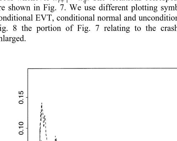
moment of the truncated innovation distribution E ZNZ)zq , these residuals should behave like an iid sample with mean zero. In Fig. 9 we show these exceedance residuals for the BMW series and qs0.95. Clearly for residuals calculated under an assumption of conditional normality the null hypothesis seems doubtful.
To test the hypothesis of mean zero we use a bootstrap test that makes no Ž
assumption about the underlying distribution of the residuals see page 224 of .
Fig. 9. Exceedance residuals for the BMW series and qs0.95. Under the null hypothesis that the
Ž .
dynamics in Eq. 1 and the tail of the innovation distribution are correctly estimated, these should have mean zero. The right graph shows clear evidence against the conditional normality assumption; the left graph shows the assumption of a conditional GPD tail is more reasonable. Note that there are only 210 normal residuals as opposed to 261 GPD residuals; refer to Table 2 to see that conditional normality overestimates the conditional quantile xt for the BMW data.
0.95
On the other hand, the GPD-based residuals are much more plausibly mean zero. In the following Table 4 we give p-values for the test applied to the GPD residuals for all five test series and various values of q. The most problematic
Ž .
series are the two indices S & P and DAX ; for the former the null hypothesis is
Table 4
p-values for a one-sided bootstrap test of the hypothesis that the exceedance residuals in the GPD case have mean zero against the alternative that the mean is greater than zero
q 0.95 0.99 0.995
S&P 0.06 0.01 0.01
DAX 0.09 0.06 0.01
BMW 0.36 0.08 0.11
USD.GBP 0.28 0.26 0.62
Ž .
rejected at the 5% level for qs0.99 and qs0.995; for the latter the null hypothesis is rejected for qs0.995. The null hypothesis is also rejected for the Gold price returns series and qs0.99. In all other cases, it is not rejected and for the BMW and USD–GBP series the hypothesis of zero-mean seems quite strongly supported.
5. Multiple day returns
tŽ .
In this section we consider estimates of xq h for h)1. Among other reasons, Ž
this is of interest if we want to obtain an estimate of the 10-day VaR as required .
by the BIS-rule from a model fitted to daily data. For GARCH-models Ž .
FXt q. . .qX NGG x is not known analytically even for a known innovation
q1 tqh t
distribution, so we adopt a simulation approach to obtaining these estimates as follows. Working with the last n negative log returns we fit as before the
Ž . Ž .
AR 1 -GARCH 1,1 model and this time we estimate both tails of the innovation
ˆ
Ž1.ˆ
Ž1. Ž .distribution F z .Z j and b are used to denote the estimated parameters of
ˆ
Ž2.ˆ
Ž2.the GPD excess distribution for the positive tail and j and b denote the corresponding parameters for the negative tail.
We simulate iid noise from the innovation distribution by a combination of bootstrap and GPD simulation according to the following algorithm which was
Ž .
also proposed independently by Danielsson and de Vries 1997c .
1. Randomly select a residual from the sample of n residuals.
ˆ
Ž1.ˆ
Ž1.4. Otherwise return the residual itself. 5. Replace residual in sample and repeat.
This gives points from the distribution
Using this composite estimate of the noise distribution and the fitted GARCH
Ž .
model we can simulate future paths xtq1, . . . , xtqh and calculate the correspond-ing cumulative sums which are simulated iid observations from our estimate for
Ž .
the distribution FXt q. . .qX NGG x . In our implementation we choose to simulate
q1 tqh t
1000 paths and to construct 1000 iid observations of the conditional h-day return. To increase precision we then apply a second round of EVT by setting a threshold at the 101st order statistic of these data and calculating GPD-based estimates of
t Ž . t Ž .
x0.95 h and x0.99 h . In principle it would also be possible to calculate estimates
t Ž . t Ž .
of S0.95 h and S0.99 h in this way, although we do not go this far.
For horizons of hs5 and hs10 days backtesting results are collected in Table 5 for the same datasets used in Table 2. We compare the Monte-Carlo method proposed above, which we again label conditional EVT, with the approach where the conditional 1-day EVT estimates are simply scaled with the square-root of the horizon h. For a given historical series x , . . . , x , with m1 m 4n, we
tŽ . 4
calculate x
ˆ
q h on days t in the set Ts n, . . . , myh and compare each estimatewith xtq1q. . .qxtqh. Under the null hypothesis of no systematic estimation error each comparison is a realization of a Bernoulli event with failure probability
Table 5
Backtesting Results: Theoretically expected number of violations and number of violations obtained
Ž .
using our approach Monte Carlo simulation from the k-day conditional distribution and square-root-of-time scaling of 1-day estimates
S&P DAX BMW $r£ Gold
hs5; length of test 7409 5141 5141 3270 3409
0.95 Quantile
Expected 371 257 257 164 170
Ž .
Conditional EVT h-day 380 247 231 185 156
Square-root-of-time 581 315 322 199 160
0.99 Quantile
Expected 74 51 51 33 34
Ž .
Conditional EVT h-day 81 46 57 44 38
Square-root-of-time 176 71 65 42 27
hs10; length of test 7405 5136 5136 3265 3404
0.95 Quantile
Expected 370 257 257 163 170
Ž .
Conditional EVT h-day 403 249 231 170 147
Square-root-of-time 623 318 315 196 163
0.99 Quantile
Expected 74 51 51 33 34
Ž .
Conditional EVT h-day 85 48 53 46 34
1yq, but we have a series of dependent comparisons because we use overlapping k-day returns. It is thus difficult to construct formal tests of violation counts, as we
did in the case of 1-day horizons. For the multiple day backtests we simply provide qualitative comparisons of expected and observed numbers of violations for the two methods.
In 16 out of 20 backtests the Monte Carlo method is closer to the expected number of violations and in all cases it performs reasonably well. In contrast, square-root-of-time seems to severely underestimate the relevant quantiles for the BMW stock returns and the two stock indices. Its performance is somewhat better for the dollar-sterling exchange rate and the price of gold.
We are not aware of a theoretical justification for a universal power law scaling
tŽ . t l
relationship of the form xq hrxqfh for conditional quantiles. However, if such a rule is to be used, our results suggest that the exponent lshould be greater than a half, certainly for stock market return series. In this context see Diebold et
Ž .
al. 1998 , who also argue against square-root-of-time scaling. Our results also cast doubt on the usefulness for conditional quantiles of a scaling law proposed by
Ž .
Danielsson and de Vries 1997c where the scaling exponent isj, the reciprocal of the tail index of the marginal distribution of the stationary time series, which typically takes values around 0.25.
6. Conclusion
The present paper is concerned with tail estimation for financial return series and, in particular, the estimation of measures of market risk such as value at risk ŽVaR or the expected shortfall. We fit GARCH-models to return data using. pseudo maximum likelihood and use a GPD-approximation suggested by extreme value theory to model the tail of the distribution of the innovations. This approach is compared to various other methods for tail estimation for financial data. Our main findings can be summarized as follows.
v We find that a conditional approach that models the conditional distribution
of asset returns against the current volatility background is better suited for VaR estimation than an unconditional approach that tries to estimate the marginal distribution of the process generating the returns. The conditional approach is vindicated by the very satisfying overall performance of our method in various backtesting experiments.
v We advocate the expected shortfall as an alternative risk measure with good
theoretical properties. This risk measure is easy to estimate in our model. A comparison of estimates for the expected shortfall using our approach and a standard GARCH-model with normal innovations shows again that the innovation distribution should be modelled by a fat-tailed distribution, preferably using EVT.
v We find that square-root-of-time scaling of one-day VaR estimates to obtain
VaR estimates for longer time horizons of 5 or 10 days does not perform well in practice, particularly for stock market returns. In contrast we propose a Monte Carlo method based on our fitted models that gives more reasonable results.
In practice, VaR estimation is often concerned with multivariate return series. We are optimistic that our Atwo-stage-methodB can be extended to multivariate series. However, a detailed analysis of this question is left for future research.
Acknowledgements
We wish to thank Paul Embrechts, Peter Buhlmann, Daniel Straumann, Neil
¨
Shephard, an anonymous referee and seminar participants at UBS-Warburg Dillon Read for interesting remarks. The data on gold-prices were obtained from the Finanzmarktdatenbank maintained by the SFB 303 at the University of Bonn. The binomial test in Section 3 was suggested by Daniel Straumann. Financial support
Ž . Ž .
from Swiss Re McNeil and from UBS Frey is gratefully acknowledged.
References
Ž .
Artzner, P., Delbaen, F., Eber, J., Heath, D., 1997. Thinking coherently. Risk 10 11 , 68–71. Artzner, P., Delbaen, F., Eber, J., Heath, D., 1999. Coherent measures of risk. Mathematical Finance 9
Ž .3 , 203–228.
Balkema, A., de Haan, L., 1974. Residual life time at great age. Annals of Probability 2, 792–804.
Ž .
Barone-Adesi, G., Bourgoin, F., Giannopoulos, K., 1998. Don’t look back. Risk 11 8 .
Basle Comittee, 1996. Overview of the Amendment of the Capital Accord to Incorporate Market Risk. Basle Committee on Banking Supervision.
Bollerslev, T., Chou, R., Kroner, K., 1992. ARCH modeling in finance. Journal of Econometrics 52, 5–59.
Brandt, A., 1986. The stochastic equation Ynq1sA Yn nqB with stationary coefficients. Advances inn
Applied Probability 18, 211–220.
Christoffersen, P., Diebold, F., Schuermann, T., 1998. Horizon problems and extreme events in financial risk management. Preprint, International Monetary Fund.
Danielsson, J., de Vries, C., 1997. Beyond the sample: extreme quantile and probability estimation. Preprint, Tinbergen Institute, Rotterdam.
Danielsson, J., de Vries, C., 1997b. Tail index and quantile estimation with very high frequency data. Journal of Empirical Finance 4, 241–257.
Danielsson, J., de Vries, C., 1997c. Value-at-Risk and extreme returns, FMG-Discussion Paper NO 273, Financial Markets Group, London School of Economics.
Ž .
Diebold, F., Schuermann, T., Hickmann, A., Inoue, A., 1998. Scale models. Risk 11, 104–107. Diebold, F., Schuermann, T., Stroughair, J., 1999. Pitfalls and opportunities in the use of extreme value
theory in risk management, Advances in Computational Finance. Kluwer Academic Publishing, Amsterdam, forthcoming.
Ž .
Duan, J.-C., 1997. Augmented GARCH p,q process and its diffusion limit. Journal of Econometrics 79, 97–127.
Ž
Duffie, D., Pan, J., 1997. An overview of value at risk. The Journal of Derivatives, 7–49, Spring:
.
1997 .
Efron, B., Tibshirani, R., 1993. An Introduction to the Bootstrap. Chapman and Hall, New York. Embrechts, P., Kluppelberg, C., Mikosch, T., 1997. Modelling Extremal Events for Insurance and¨
Finance. Springer, Berlin.
Ž .
Embrechts, P., Resnick, S., Samorodnitsky, G., 1998. Living on the edge. Risk Magazine 11 1 , 96–100.
Embrechts, P., Resnick, S., Samorodnitsky, G., 1999. Extreme value theory as a risk management tool.
Ž .
North American Actuarial Journal 3 2 , 30–41, forthcoming.
Gnedenko, B., 1943. Sur la distribution limite du terme maximum d’une serie aleatoire. Annals of´ ´
Mathematics 44, 423–453.
Gourieroux, C., 1997. ARCH-models and financial applications, Springer Series in Statistics. Springer,´
New York.
Hill, B., 1975. A simple general approach to inference about the tail of a distribution. Annals of Statistics 3, 1163–1174.
Longin, F., 1997. Beyond the VaR, Discussion Paper 97-011, CERESSEC.
Longin, F., 1997. From value at risk to stress testing, the extreme value approach, Discussion Paper 97-004, CERESSEC.
McNeil, A., 1997. Estimating the tails of loss severity distributions using extreme value theory. ASTIN Bulletin 27, 117–137.
McNeil, A., 1998. Calculating Quantile Risk Measures for Financial Return Series using Extreme Value Theory, preprint, ETH Zurich.¨
McNeil, A., Saladin, T., 1997. The peaks over thresholds method for estimating high quantiles of loss distributions. Proceedings of XXVIIth International ASTIN Colloquium, Cairns, Australia. pp. 23–43.
Muller, O., Dacarogna, M., Dave, R., Olsen, R., Pictet, O., von Weizsacker, J., 1997. Volatilities of¨ ´ ¨
different time resolutions — analyzing the dynamics of market components. Journal of Empirical
Ž .
Finance 4 2–3 , 213–240.
Pagan, A., 1996. The econometrics of financial markets. Journal of Empirical Finance 3, 15–102. Pickands, J., 1975. Statistical inference using extreme order statistics. The Annals of Statistics 3,
119–131.
Resnick, S., Starica, C., 1995. Consistency of Hill’s estimator for dependent data. Journal of Appliedˇ ˇ
Probability 32, 239–267.
Resnick, S., Starica, C., 1996. Tail index estimation for dependent data, Technical Report, School ofˇ ˇ
ORIE, Cornell University.
RiskMetrics, 1995. RiskMetrics Technical Document. 3rd edn. J.P. Morgan.
Shephard, N., 1996. Statistical aspects of ARCH and stochastic volatility. In: Cox, D., Hinkley, D.,
Ž .
Barndorff-Nielsen, O. Eds. , Time Series Models in Econometrics, Finance and other Fields. Chapman and Hall, London, pp. 1–55.