www.elsevier.com / locate / econbase
Effects of monetary policy shocks on the trade balance in small
open European countries
*
Soyoung Kim
Department of Economics, 225b DKH, University of Illinois at Urbana–Champaign, 1407 W. Gregory Dr.,
Urbana, IL 61801, USA
Received 17 April 2000; accepted 7 November 2000
Abstract
The effects of monetary policy shocks on trade balance (in volume, unit value, and total nominal value) are examined in France, Italy, and the UK using VAR models. The results are consistent with the expenditure-switching effect, but there is little evidence of the J-curve effect. 2001 Elsevier Science B.V. All rights reserved.
Keywords: Monetary policy shocks; Expenditure-switching effect; VAR; Trade balance; Terms of trade
JEL classification: C30; E52; F41
1. Introduction
This paper documents empirical evidence of the effects of monetary policy shocks on the trade balance in small open European countries (Italy, France, and the UK) for the recent period. First, we document empirical evidence of the effects of monetary policy shocks on the trade balance over time. Second, we examine the effects of monetary policy shocks on related variables such as terms of trade, real exchange rate, and nominal exchange rate to better understand detailed monetary transmission mechanisms. Third, we examine the magnitude of the contribution of monetary policy shocks to trade statistics. Finally, based on the evidence, we address several questions of interests to academics in the field of open economy macro and monetary economics and to policy makers.
There have been many empirical investigations in this area. However, the evidence is based on specific theoretical models, which may not serve as data-oriented empirical evidence or the evidence
*Tel.:11-217-356-9291; fax: 11-217-333-1398.
E-mail address: [email protected] (S. Kim).
1
provides the limited evidence on the detailed transmission mechanism. In addition, there is little empirical evidence on small open economies such as Italy, France, and UK.
Regarding empirical methodology, newly developed models in the VAR literature on identifying monetary policy shocks are employed. Specifically, we modify the VAR models which have been successful in identifying monetary policy shocks in small open economies such as in the work of Kim (1999) and Kim and Roubini (2000). These models employ minimal identifying restrictions which do not depend on specific theoretical models. Consequently, we are able to document data-oriented evidence on international monetary transmissions.
Section 2 explains the empirical model. Section 3 discusses the empirical evidence of the effects of the monetary policy shocks on the trade balance. Section 4 summarizes the results.
2. Empirical model
In the model, the data vector is hR, M, CPI, IP, WR, CMPW, X1, X2j, where R is the short term interest rate, M is a monetary aggregate, CPI is the consumer price index, IP is industrial production, WR is the world short-term interest rate, CMPW is the world export commodity price index in terms
2
of domestic currency, and X1 and X2 are trade statistics. The first four variables are essential in identifying monetary policy shocks. The next two variables are included in order to control for the systematic component of the policy rule (inflationary and world shocks) and isolate ‘exogenous’
3
monetary policy changes.
The empirical model imposes (non-recursive) zero restrictions on the contemporaneous structural parameters. For the restrictions on the contemporaneous structural parameters, we follow the general idea of Kim (1999) and Kim and Roubini (2000). Note that we do not impose any restrictions on lagged structural parameters. The following equations summarize our identification scheme.
1 g12 0 0 g15 g16 0 0 R R eR
Examples of past works are studies in Bryant et al. (1988), Betts and Devereux (2000), Kim and Roubini (2000), Clarida and Gali (1994), among many others.
2
We use M02 for the UK and M1 for France and Italy. We use the average of the US Federal Funds rate and the German short-term interest rate as the proxy for the world interest rate. As suggested by Kim and Roubini (2000) and Clarida et al. (1997), it is important to control for the US and German monetary policy for these European countries.
3
where e , e , eR M CPI, e , eIP WR, eCMPW, eX1, and eX2 are structural disturbances. In particular, eR is interpreted as monetary policy shocks.
The first equation in (1) is the monetary reaction function. The monetary authority is assumed to set the interest rate after observing the current value of money, CMPW, and the world interest rate but not the current values of output nor the price level. This assumption is based on the fact that we assume information delays, such that data on money, commodity price, and the world interest rate are
4
available within a month, but data on output and the price level are not. The second equation is a money demand equation, representing that the demand for real money balances depends on real income and the nominal interest rate.
The fifth equation assumes that the world interest rate is contemporaneously exogenous to all variables in the system, that is, an individual small open economy cannot affect the world interest rate contemporaneously. The third and fourth equations represent the sluggish real sector. Real activity is
5
assumed to respond to monetary policy and financial signals only with a lag.
The sixth, seventh, and eight equations are (normalized) blocks of equations that are contempora-neously affected by all variables in the system. The world export commodity price equation is assumed to be an arbitrage equation, which describes a kind of financial market equilibrium. We do not impose any restrictions on the equations for X1 and X2 since we are interested in how X1 and X2 respond.
Data are gathered monthly. They are found in the IFS database except for M02 of the UK, which is from the Bank of England’s Web page. The estimation periods are 1976:9–1996:6 for France,
6
1981:6–1996:12 for Italy, and 1979:1–1996:12 for the UK. All variables were used in logarithm form except for interest rates. Complete seasonal dummies are used in all estimations. Six lags were assumed. We skip the detailed estimation method on the structural VAR model since it is
well-7
documented in the past studies.
Impulse responses of the first six variables to monetary policy shocks in our system do not show any puzzling responses (such as price puzzle). In addition, the likelihood ratio test of the over-identifying restrictions suggests that the over-over-identifying restrictions are not rejected at any conventional significance level in each case.
3. International monetary transmission mechanism
We employ the dataset which decomposes the total nominal values (in terms of each country’s currency) of exports and imports into the volumes and the unit values. Three different pairs of X1 and
4
For France and Italy, we give another zero restriction on g , as Kim and Roubini (2000) suggest.12 5
This assumption has been widely used by previous researchers, for example, Sims and Zha (1996), Kim (1999), Christiano et al. (1998), Gordon and Leeper (1994), Kim and Roubini (2000). Additional restrictions of g3550 and g3550 do not affect the results much.
6
´
For France, we choose the starting date of 1976:9, when the Barre plan of price stabilization starts (see Melitz, 1991). We also estimated the model from 1979:3 when the ERM launched, but the results are similar. For Italy, we choose the starting date of 1981:6, when the Bank of Italy divorces from the Treasury (see Passacantando, 1996). We also estimated the model from 1979:3, but the results are similar. For the UK, we choose the starting date of 1979:1, around when Thatcher assumed power, fighting inflation became a clear policy objective, and the ERM launched. We also estimated the model starting from 1979:6 and 1979:3, which are the exact dates of those events, but the results are similar.
7
X2 are included. The first includes the volumes, the second includes the unit values, and the third includes the nominal values. Both exports (X1) and imports (X2) are included in each system. The difference between exports and imports is reported in each case. All variables are included in the form of a logarithm. We proxy the differences in the volumes of exports and imports as the trade balance in real terms and the differences in the unit values as the terms of trade (export price / import price). Finally, to infer detailed mechanisms, we include another pair of variables, nominal (X1) and real
8
(X2) exchange rates, in a separate system.
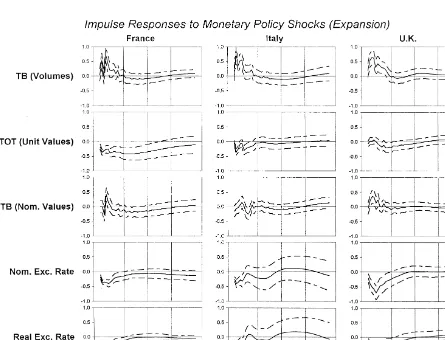
Fig. 1 reports the impulse responses to one standard-deviation monetary policy shocks (expansion) in each country with one standard error band over 4 years. In each graph, vertical lines are inserted each year after the shocks. First, the volume of the trade balance (the real value) increases initially, but returns to the initial level in about a year. The peak increase is found within 6 months. Second, the unit value of the trade balance (the terms of trade) decreases. The responses are slightly different in each country. Third, the responses of the total nominal values of the trade balance are much different
Fig. 1. Impulse responses to monetary policy shocks. 8
across countries, depending on the size and the persistency of the volume and the value effects. In general, they are small, reflecting the opposite movements of the value and the volume effects. Finally, the nominal and real exchange rates depreciate. Note that the responses of the nominal and real exchange rates are similar while the responses of two exchange rates and the terms of trade are somewhat different. The terms of trade decrease is more delayed than the exchange rate depreciation. The peak exchange rate depreciation is found in 2–5 months while the peak decrease in the terms of trade is found in 6 months to 1 year.
First, we compare the impulse responses with theoretical predictions. The basic predictions of the traditional Mundell–Flemming–Dornbusch (MFD) model are the following. A monetary expansion leads to a depreciation in the nominal exchange rate and a deterioration of the terms of trade, which results in an improvement of the trade balance — the expenditure-switching effect. However, a monetary expansion also stimulates domestic demand, which may lead to an increase in imports and a worsening of the trade balance — the income-absorption effect. These two effects move the trade balance in opposite directions. The movements of the trade balance are determined by the dominant
9
effect.
In general, the expenditure-switching effect seems to dominate the income-absorption effect. The impulse responses are consistent with the expenditure-switching effect. A monetary expansion leads a nominal exchange rate depreciation and a deterioration of the terms of trade (the unit value). As a result, the volume of the trade balance increases.
We find little evidence of the J-curve effect. The J-curve effect suggests that an exchange rate depreciation may result in an initial nominal trade balance deficit (in terms of the domestic currency) since the value effects are immediate but the volume effects are delayed. The impulse responses suggest that the volume effects are not much delayed while the value effects are not immediate. The volume of the trade balance starts to increase immediately, and the peak increase is found in 2–5 months. The value of the trade balance also starts to increase immediately, but the peak increase is found only in about 6 months to 1 year. Though the exchange rate response is more immediate, the terms of trade reflects the nominal exchange rate change with a delay, which may be one reason that the J-curve effect is not found.
Next, we discuss the implications of our results on theoretical modeling. First, to explain the negative correlation between trade balance and output (for example, see Backus and Kehoe (1992) and Baxter (1996)), it is important to introduce structural shocks other than monetary shocks in a theoretical model since monetary shocks generate the positive correlation. Second, a separate modeling of the real exchange rate and the terms of trade may be important in analyzing the international monetary transmission (for example, Obstfeld and Rogoff (1995) and Betts and Devereux (2000)) since the responses of the real exchange rate and the terms of trade are somewhat different.
We also compare the results for the US with the results for the small open European economies studied here. Kim (2000) reports that a typical US monetary expansion leads to a short-run worsening of the trade balance (in real terms or the volume measure), but a long-run persistent (up to 5–6 years) improvement of the trade balance. In contrast, the trade balance (the volume measure) improves within a few months, but the improvement is short-lived (about 1 year) in these European countries.
9
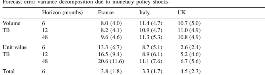
Table 1
Forecast error variance decomposition due to monetary policy shocks Horizon (months) France Italy UK
Volume 6 8.0 (4.0) 11.4 (4.7) 10.7 (5.0)
TB 12 8.2 (4.1) 10.9 (4.7) 11.0 (4.9)
48 9.6 (4.6) 11.3 (5.3) 10.8 (4.9)
Unit value 6 13.3 (6.7) 8.7 (5.1) 2.6 (2.4)
TB 12 16.5 (9.4) 8.9 (6.1) 5.2 (4.6)
48 20.6 (11.6) 11.1 (7.6) 6.7 (5.6)
Total 6 3.8 (1.8) 3.3 (1.7) 4.5 (2.3)
TB 12 6.4 (4.1) 5.3 (2.6) 5.1 (2.5)
48 7.6 (5.2) 7.1 (4.2) 5.7 (3.0)
One difference in the transmission mechanism is due to the persistency of the terms of trade deterioration. In the Kim (2000) results, the terms of trade deterioration is persistent in response the US expansionary monetary policy shocks, but it is short-lived in response to these European
10
countries’ expansionary monetary policy shocks.
Table 1 reports the forecast error variance decomposition of the unit value, the volume, and the total nominal value of the trade balance in each country. The numbers in the parentheses are standard errors. In general, the contribution of monetary policy shocks to each measure of the trade balance is small in most cases. Since the role of monetary policy shocks is limited in explaining the observed high volatility of the trade balance and the terms of trade (for example, see Baxter (1996) and Backus et al. (1992)), introducing monetary policy shocks in the theoretical model do not seem to be the best way to match the high volatility in the data.
Finally, we may loose some information on the interactions among trade statistics based on our estimation methods since we include only two trade statistics each time. By changing combinations of trade statistics, we examine the importance of these interactions. In most cases, the impulse responses are similar.
4. Conclusion
In France, Italy, UK, the effects of monetary policy shocks on trade balance are consistent with expenditure-switching effect, but there is little evidence of J-curve effect.
Acknowledgements
I thank Andre Baretto and Min Jung Chae for research assistance. I acknowledge financial support from UIUC Research Board. I thank Hyungsoo Park for useful suggestions. Some parts of this
10
research was conducted while I was a visiting research fellow at the Bank of Korea. The usual disclaimer applies.
References
Backus, D.K., Kehoe, P.J., 1992. International evidence on the historical properties of business cycles. American Economic Review 82, 864–888.
Backus, D.K., Kehoe, P.J., Kydland, F.E., 1992. International real business cycles. Journal of Political Economy 100, 745–775.
Baxter, M., 1996. International trade and business cycles. In: Grossman, G., Rogoff, K. (Eds.). Handbook of International Economics, Vol. III. North Holland, Amsterdam.
Betts, C., Devereux, M.B., 2000. Exchange rate dynamics in a model of pricing-to-market. Journal of International Economics 50, 215–244.
Bryant, R., Hooper, P., Mann, C., 1988. Empirical Macroeconomics For Independent Economies. Brookings, Washington, DC.
Christiano, L., Eichenbaum, M., Evans, C., 1998. Monetary Policy Shocks: What Have We Learned and To What End. NBER Working Paper No. 6400.
Clarida, R., Gali, M., 1994. Sources of Real Exchange Rate Fluctuations: How Important Are Nominal Shocks. Carnegie–Rochester Series on Public Policy.
Clarida, R., Gali, J., Gertler, M., 1997. Monetary Policy Rules in Practice: Some International Evidence. NBER Working Paper No. 6254.
Gordon, D.B., Leeper, E.M., 1994. The dynamic impacts of monetary policy: An exercise in tentative identification. Journal of Political Economy 102, 228–247.
Kim, S., 1999. Do monetary policy shocks matter in the G-7 countries? Using common identifying assumptions about monetary policy across countries. Journal of International Economics 48, 387–412.
Kim, S., 2000. International transmission of the US monetary policy shocks: Evidence from VARs. Journal of Monetary Economics 45 (forthcoming).
Kim, S., Roubini, N., 2000. Exchange rate anomalies in the industrial countries: A solution with a structural VAR approach. Journal of Monetary Economics 45, 561–586.
´
Melitz, J., 1991. Monetary Policy in France. CEPR Discussion Paper No. 509.
Obstfeld, M., Rogoff, K., 1995. Exchange rate dynamics redux. Journal of Political Economy 103, 624–660.
Passacantando, F., 1996. Building an Institutional Framework For Monetary Stability: The Case of Italy. BNL Quarterly Review.
Sims, C.A., 1992. Interpreting the macroeconomic time series facts: The effects of monetary policy. European Economic Review 36, 975–1000.
Sims, C.A., Zha, T., 1996. Does Monetary Policy Generate Recessions? Using Less Aggregate Price Data To Identify Monetary Policy. Working Paper. Yale University, Connecticut.