Disk-Based
Algorithms for
Disk-Based
Algorithms for
Big Data
Christopher G. Healey
North Carolina State University
6000 Broken Sound Parkway NW, Suite 300 Boca Raton, FL 33487-2742
© 2017 by Taylor & Francis Group, LLC
CRC Press is an imprint of Taylor & Francis Group, an Informa business
No claim to original U.S. Government works
Printed on acid-free paper Version Date: 20160916
International Standard Book Number-13: 978-1-138-19618-6 (Hardback)
This book contains information obtained from authentic and highly regarded sources. Reasonable efforts have been made to publish reliable data and information, but the author and publisher cannot assume responsibility for the validity of all materials or the consequences of their use. The authors and publishers have attempted to trace the copyright holders of all material reproduced in this publication and apologize to copyright holders if permission to publish in this form has not been obtained. If any copyright material has not been acknowledged please write and let us know so we may rectify in any future reprint.
Except as permitted under U.S. Copyright Law, no part of this book may be reprinted, reproduced, transmitted, or utilized in any form by any electronic, mechanical, or other means, now known or hereafter invented, including photocopying, microfilming, and recording, or in any information stor-age or retrieval system, without written permission from the publishers.
For permission to photocopy or use material electronically from this work, please access www.copy-right.com (http://www.copywww.copy-right.com/) or contact the Copyright Clearance Center, Inc. (CCC), 222 Rosewood Drive, Danvers, MA 01923, 978-750-8400. CCC is a not-for-profit organization that pro-vides licenses and registration for a variety of users. For organizations that have been granted a photo-copy license by the CCC, a separate system of payment has been arranged.
Trademark Notice: Product or corporate names may be trademarks or registered trademarks, and are used only for identification and explanation without intent to infringe.
Visit the Taylor & Francis Web site at http://www.taylorandfrancis.com
To my sister, the artist
To my parents
List of Tables
xv
List of Figures
xvii
Preface
xix
C
hapter
1
Physical Disk Storage
1
1.1 PHYSICAL HARD DISK 2
1.2 CLUSTERS 2
1.2.1
Block Allocation
3
1.3 ACCESS COST 4
1.4 LOGICAL TO PHYSICAL 5
1.5 BUFFER MANAGEMENT 6
C
hapter
2
File Management
9
2.1 LOGICAL COMPONENTS 9
2.1.1
Positioning Components
10
2.2 IDENTIFYING RECORDS 12
2.2.1
Secondary Keys
12
2.3 SEQUENTIAL ACCESS 13
2.3.1
Improvements
13
2.4 DIRECT ACCESS 14
2.4.1
Binary Search
15
2.5 FILE MANAGEMENT 16
2.5.1
Record Deletion
16
2.5.2
Fixed-Length Deletion
17
2.5.3
Variable-Length Deletion
19
2.6 FILE INDEXING 20
2.6.1
Simple Indices
20
2.6.2
Index Management
21
2.6.3
Large Index Files
22
2.6.4
Secondary Key Index
22
2.6.5
Secondary Key Index Improvements
24
C
hapter
3
Sorting
27
3.1 HEAPSORT 27
3.2 MERGESORT 32
3.3 TIMSORT 34
C
hapter
4
Searching
37
4.1 LINEAR SEARCH 37
4.2 BINARY SEARCH 38
4.3 BINARY SEARCH TREE 38
4.4 k-d TREE 40
4.4.1
k-d Tree Index
41
4.4.2
Search
43
4.4.3
Performance
44
4.5 HASHING 44
4.5.1
Collisions
44
4.5.2
Hash Functions
45
4.5.3
Hash Value Distributions
46
4.5.4
Estimating Collisions
47
4.5.5
Managing Collisions
48
4.5.6
Progressive Overflow
48
4.5.7
Multirecord Buckets
50
C
hapter
5
Disk-Based Sorting
53
5.1 DISK-BASED MERGESORT 54
5.1.1
Basic Mergesort
54
5.1.2
Timing
55
5.1.3
Scalability
56
5.3 MORE HARD DRIVES 57
5.4 MULTISTEP MERGE 58
5.5 INCREASED RUN LENGTHS 59
5.5.1
Replacement Selection
59
5.5.2
Average Run Size
61
5.5.3
Cost
61
5.5.4
Dual Hard Drives
61
C
hapter
6
Disk-Based Searching
63
6.1 IMPROVED BINARY SEARCH 63
6.1.1
Self-Correcting BSTs
64
6.1.2
Paged BSTs
64
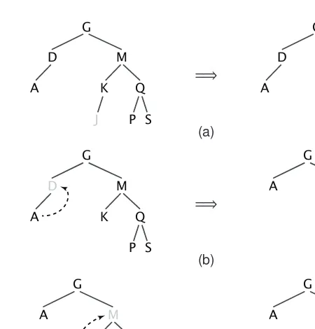
6.2 B-TREE 66
6.2.1
Search
68
6.2.2
Insertion
68
6.2.3
Deletion
70
6.3 B∗TREE 71
6.4 B+ TREE 73
6.4.1
Prefix Keys
74
6.5 EXTENDIBLE HASHING 75
6.5.1
Trie
76
6.5.2
Radix Tree
76
6.6 HASH TRIES 76
6.6.1
Trie Insertion
78
6.6.2
Bucket Insertion
79
6.6.3
Full Trie
79
6.6.4
Trie Size
79
6.6.5
Trie Deletion
80
6.6.6
Trie Performance
81
C
hapter
7
Storage Technology
83
7.1 OPTICAL DRIVES 84
7.1.1
Compact Disc
84
7.1.2
Digital Versatile Disc
85
7.2 SOLID STATE DRIVES 86
7.2.1
Floating Gate Transistors
87
7.2.2
Read–Write–Erase
88
7.2.3
SSD Controller
88
7.2.4
Advantages
89
7.3 HOLOGRAPHIC STORAGE 89
7.3.1
Holograms
89
7.3.2
Data Holograms
91
7.3.3
Commercialization
91
7.4 MOLECULAR MEMORY 91
7.5 MRAM 93
C
hapter
8
Distributed Hash Tables
95
8.1 HISTORY 96
8.2 KEYSPACE 96
8.3 KEYSPACE PARTITIONING 97
8.4 OVERLAY NETWORK 97
8.5 CHORD 97
8.5.1
Keyspace
98
8.5.2
Keyspace Partitioning
98
8.5.3
Overlay Network
99
8.5.4
Addition
100
8.5.5
Failure
100
C
hapter
9
Large File Systems
101
9.1 RAID 101
9.1.1
Parity
102
9.2 ZFS 103
9.2.1
Fault Tolerance
104
9.2.2
Self-Healing
104
9.2.3
Snapshots
104
9.3 GFS 105
9.3.1
Architecture
105
9.3.2
Master Metadata
106
9.3.4
Fault Tolerance
107
9.4 HADOOP 107
9.4.1
MapReduce
108
9.4.2
MapReduce Implementation
109
9.4.3
HDFS
110
9.4.4
Pig
111
9.4.5
Hive
115
9.5 CASSANDRA 116
9.5.1
Design
117
9.5.2
Improvements
119
9.5.3
Query Language
120
9.6 PRESTO 121
C
hapter
10
NoSQL Storage
125
10.1 GRAPH DATABASES 126
10.1.1 Neo4j
126
10.1.2 Caching
128
10.1.3 Query Languages
129
10.2 DOCUMENT DATABASES 130
10.2.1 SQL Versus NoSQL
131
10.2.2 MongoDB
132
10.2.3 Indexing
134
10.2.4 Query Languages
135
A
ppendix
A
Order Notation
137
A.1
Θ
-NOTATION 137A.2
O-NOTATION
138A.3
Ω
-NOTATION 139A.4 INSERTION SORT 139
A.5 SHELL SORT 141
A
ppendix
B
Assignment 1: Search
145
B.1 KEY AND SEEK LISTS 146
B.3 IN-MEMORY SEQUENTIAL SEARCH 147
B.4 IN-MEMORY BINARY SEARCH 147
B.5 ON-DISK SEQUENTIAL SEARCH 148
B.6 ON-DISK BINARY SEARCH 148
B.7 PROGRAMMING ENVIRONMENT 149
B.7.1
Reading Binary Integers
149
B.7.2
Measuring Time
150
B.7.3
Writing Results
150
B.8 SUPPLEMENTAL MATERIAL 151
B.9 HAND-IN REQUIREMENTS 151
A
ppendix
C
Assignment 2: Indices
153
C.1 STUDENT FILE 153
C.2 PROGRAM EXECUTION 155
C.3 IN-MEMORY PRIMARY KEY INDEX 155
C.4 IN-MEMORY AVAILABILITY LIST 156
C.4.1
First Fit
157
C.4.2
Best Fit
157
C.4.3
Worst Fit
157
C.5 USER INTERFACE 158
C.5.1
Add
158
C.5.2
Find
159
C.5.3
Del
159
C.5.4
End
159
C.6 PROGRAMMING ENVIRONMENT 159
C.6.1
Writing Results
160
C.7 SUPPLEMENTAL MATERIAL 160
C.8 HAND-IN REQUIREMENTS 161
A
ppendix
D
Assignment 3: Mergesort
163
D.1 INDEX FILE 163
D.2 PROGRAM EXECUTION 164
D.3 AVAILABLE MEMORY 164
D.4 BASIC MERGESORT 164
D.6 REPLACEMENT SELECTION MERGESORT 166
D.7 PROGRAMMING ENVIRONMENT 167
D.7.1
Measuring Time
167
D.7.2
Writing Results
168
D.8 SUPPLEMENTAL MATERIAL 168
D.9 HAND-IN REQUIREMENTS 168
A
ppendix
E
Assignment 4: B-Trees
171
E.1 INDEX FILE 171
E.2 PROGRAM EXECUTION 172
E.3 B-TREE NODES 172
E.3.1
Root Node O
ff
set
173
E.4 USER INTERFACE 173
E.4.1
Add
174
E.4.2
Find
174
E.4.3
175
E.4.4
End
175
E.5 PROGRAMMING ENVIRONMENT 175
E.6 SUPPLEMENTAL MATERIAL 176
E.7 HAND-IN REQUIREMENTS 176
1.1 Hard Drive Specs 4
1.2 Access Cost 5
2.1 Delimiter Methods 11
2.2 Linear vs. Binary Speedup 15
2.3 Variable Length Index 21
2.4 Secondary Key Index 23
2.5 Boolean Logic 24
2.6 Alternative Secondary Index 25
3.1 Sort Performance 36
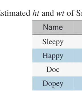
4.1 Heights and Weights 41
4.2 Collision Rate 48
5.1 Mergesort Scalability 56
5.2 Mergesort Memory Increase 58
5.3 Replacement Selection 60
9.1 Cassandra Terminology 120
10.1 Three relational tables containing various information about
cus-tomer orders 132
1.1 Hard Disk Drive 1
1.2 Drive Components 3
2.1 File Servers 9
2.2 Fields, Arrays, Records 10
2.3 Fixed-Length Deletion 18
3.1 Sorting 27
3.2 Tournament Sort 28
3.3 Heap Construction 30
3.4 Heap Tree 31
3.5 Mergesort 33
3.6 Timsort Run Stack 35
4.1 Search Field 37
4.2 BST Deletion 40
4.3 k-d Tree 42
4.4 k-d Tree Subdivision 43
4.5 Progressive Overflow 49
5.1 Mergesort Visualization 53
6.1 Credit Cards 63
6.2 Paged BST 64
6.3 Character Paged BST 66
6.4 Character B-Tree 67
6.5 Order-1001 B-Tree 67
6.6 B-Tree Insertion 69
6.7 B-Tree Deletion 70
6.8 B∗Tree Insertion 72
6.9 B+Tree 73
6.10 Radix Tree 76
6.11 Hash Trie 77
6.12 Bucket Insertion 78
6.13 Trie Extension 78
6.14 Trie Deletion 80
7.1 DVD-RW Drive 83
7.2 Blu-ray Disc 84
7.3 FG Transistor 87
7.4 Holograms 90
7.5 Rotaxane 92
7.6 Spin-Torque Transfer 93
8.1 Botnet Visualization 95
8.2 Chord Keyspace 98
9.1 Hadoop Logo 101
9.2 Hadoop Cluster 108
9.3 Cassandra Cluster 117
9.4 Presto Architecture 122
10.1 Tweet Graph 125
10.2 Friend Graph 126
10.3 Neo4j Store Files 127
10.4 MongonsFile 133
10.5 Mongo Extents 134
10.6 Mongo B-Tree Node 135
A.1 Order Graphs 137
A.2 Θn2Graph 138
B.1 Assignment 1 145
C.1 Assignment 2 153
D.1 Assignment 3 163
This book is a product of recent advances in the areas of “big data,” data analytics, and the underlying file systems and data management algorithms needed to support the storage and analysis of massive data collections.
We have offered anAdvanced File Structurescourse for senior undergraduate and graduate students for many years. Until recently, it focused on a detailed exploration of advanced in-memory searching and sorting techniques, followed by an extension of these foundations to disk-based mergesort, B-trees, and extendible hashing.
About ten years ago, new file systems, algorithms, and query languages like the Google and Hadoop file systems (GFS/HDFS), MapReduce, and Hive were intro-duced. These were followed by database technologies like Neo4j, MongoDB, Cas-sandra, and Presto that are designed for new types of large data collections. Given this renewed interest in disk-based data management and data analytics, I searched for a textbook that covered these topics from a theoretical perspective. I was unable to find an appropriate textbook, so I decided to rewrite the notes for theAdvanced File Structurescourse to include new and emerging topics in large data storage and analytics. This textbook represents the current iteration of that effort.
The content included in this textbook was chosen based of a number of basic goals:
• provide theoretical explanations for new systems, techniques, and databases
like GFS, HDFS, MapReduce, Cassandra, Neo4j, and MongoDB,
• preface the discussion of new techniques with clear explanations of traditional
algorithms like mergesort, B-trees, and hashing that inspired them,
• explore the underlying foundations of different technologies, and demonstrate
practical use cases to highlight where a given system or algorithm is well suited, and where it is not,
• investigate physical storage hardware like hard disk drives (HDDs), solid-state
drives (SSDs), and magnetoresistive RAM (MRAM) to understand how these technologies function and how they could affect the complexity, performance, and capabilities of existing storage and analytics algorithms, and
• remain accessible to both senior-level undergraduate and graduate students.
To achieve these goals, topics are organized in a bottom-up manner. We begin with the physical components of hard disks and their impact on data management,
since HDDs continue to be common in large data clusters. We examine how data is stored and retrieved through primary and secondary indices. We then review dif-ferent in-memory sorting and searching algorithms to build a foundation for more sophisticated on-disk approaches.
Once this introductory material is presented, we move to traditional disk-based sorting and search techniques. This includes different types of on-disk mergesort, B-trees and their variants, and extendible hashing.
We then transition to more recent topics: advanced storage technologies like SSDs, holographic storage, and MRAM; distributed hash tables for peer-to-peer (P2P) storage; large file systems and query languages like ZFS, GFS/HDFS, Pig, Hive, Cassandra, and Presto; and NoSQL databases like Neo4j for graph structures and MongoDB for unstructured document data.
This textbook was not written in isolation. I want to thank my colleague and friend Alan Tharp, author ofFile Organization and Processing, a textbook that was used in our course for many years. I would also like to recognize Michael J. Folk, Bill Zoellick, and Greg Riccardi, authors ofFile Structures, a textbook that provided inspiration for a number of sections in my own notes. Finally, Rada Chirkova has used my notes as they evolved in her section ofAdvanced File Structures, providing additional testing in a classroom setting. Her feedback was invaluable for improving and extending the topics the textbook covers.
I hope instructors and students find this textbook useful and informative as a starting point for their own investigation of the exciting and fast-moving area of storage and algorithms for big data.
Physical Disk Storage
FIGURE 1.1
The interior of a hard disk drive showing two platters, read
/
write
heads on an actuator arm, and controller hardware
M
ASS STORAGE for computer systems originally used magnetic tape to record information. Remington Rand, manufacturer of the Remington type-writer and the UNIVAC mainframe computer (and originally part of the Remington Arms company), built the first tape drive, the UNISERVO, as part of a UNIVAC sys-tem sold to the U.S. Census Bureau in 1951. The original tapes were 1,200 feet long and held 224KB of data, equivalent to approximately 20,000 punch cards. Although popular until just a few years ago due to their high storage capacity, tape drives are inherently linear in how they transfer data, making them inefficient for anything other than reading or writing large blocks of sequential data.Hard disk drives (HDDs) were proposed as a solution to the need for random ac-cess secondary storage in real-time accounting systems. The original hard disk drive, the Model 350, was manufactured by IBM in 1956 as part of their IBM RAMAC
(Random Access Method of Accounting and Control) computer system. The first RAMAC was sold to Chrysler’s Motor Parts division in 1957. It held 5MB of data on fifty 24-inch disks.
HDDs have continued to increase their capacity and lower their cost. A modern hard drive can hold 3TB or more of data, at a cost of about $130, or $0.043/GB. In spite of the emergence of other storage technologies (e.g., solid state flash memory), HDDs are still a primary method of storage for most desktop computers and server installations. HDDs continue to hold an advantage in capacity and cost per GB of storage.
1.1
PHYSICAL HARD DISK
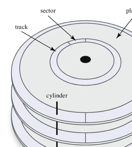
Physical hard disk drives use one or more circular platters to store information ( Fig-ure 1.1). Each platter is coated with a thin ferromagnetic film. The direction of mag-netization is used to represent binary 0s and 1s. When the drive is powered, the platters are constantly rotating, allowing fixed-position heads to read or write infor-mation as it passes underneath. The heads are mounted on an actuator arm that allows them to move back and forth over the platter. In this way, an HDD is logically divided in a number of different regions (Figure 1.2).
• Platter.A non-magnetic, circular storage surface, coated with a ferromagnetic
film to record information. Normally both the top and the bottom of the platter are used to record information.
• Track.A single circular “slice” of information on a platter’s surface.
• Sector.A uniform subsection of a track.
• Cylinder.A set of vertically overlapping tracks.
An HDD is normally built using a stack of platters. The tracks directly above and below one another on successive platters form a cylinder. Cylinders are important, because the data in a cylinder can be read in one rotation of the platters, without the need to “seek” (move) the read/write heads. Seeking is usually the most expensive operation on a hard drive, so reducing seeks will significant improve performance.
Sectors within a track are laid out using a similar strategy. If the time needed to process a sector allowsnadditional sectors to rotate underneath the disk’s read/write heads, the disk’s interleave factor is 1 :n. Eachlogicalsector is separated byn po-sitions on the track, to allow consecutive sectors to be read one after another without any rotation delay. Most modern HDDs are fast enough to support a 1 : 1 interleave factor.
1.2
CLUSTERS
platter sector
track
cylinder
FIGURE 1.2
A hard disk drive’s platters, tracks, sectors, and cylinders
contiguous group of sectors, allowing the data in a cluster to be read in a single seek. This is designed to improve efficiency.
An OS’s file allocation table (FAT) binds the sectors to their parent clusters, al-lowing a cluster to be decomposed by the OS into a set of physical sector locations on the disk. The choice of cluster size (in sectors) is a tradeoff: larger clusters pro-duce fewer seeks for a fixed amount of data, but at the cost of more space wasted, on average, within each cluster.
1.2.1 Block Allocation
Rather than using sectors, some OSs allowed users to store data in variable-sized “blocks.” This meant users could avoid sector-spanning or sector fragmentation is-sues, where data either won’t fit in a single sector, or is too small to fill a single sector. Each block holds one or more logical records, called theblocking factor. Block allo-cation often requires each block to be preceded by a count defining the block’s size in bytes, and a key identifying the data it contains.
• blocking requires an application and/or the OS to manage the data’s
organiza-tion on disk, and
• blocking may preclude the use of synchronization techniques supported by
generic sector allocation.
1.3
ACCESS COST
The cost of a disk access includes
1. Seek.The time to move the HDD’s heads to the proper track. On average, the head moves a distance equal to1
3of the total number of cylinders on the disk.
2. Rotation.The time to spin the track to the location where the data starts. On average, a track spins1
2a revolution.
3. Transfer.The time needed to read the data from the disk, equal to the number of bytes read divided by the number of bytes on a track times the time needed to rotate the disk once.
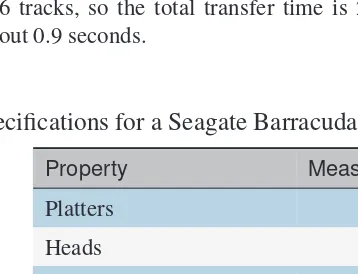
For example, suppose we have an 8,515,584 byte file divided into 16,632 sectors of size 512 bytes. Given a 4,608-byte cluster holding 9 sectors, we need a sequence of 1,848 clusters occupying at least 264 tracks, assuming a Barracuda HDD with sixty-three 512-byte sectors per track, or 7 clusters per track. Recall also the Barracuda has an 8 ms seek, 4 ms rotation delay, spins at 7200 rpm (120 revolutions per second), and holds 6 tracks per cylinder (Table 1.1).
In the best-case scenario, the data is stored contiguously on individual cylinders. If this is true, reading one track will load 63 sectors (9 sectors per cluster times 7 clusters per track). This involves a seek, a rotation delay, and a transfer of the entire track, which requires 20.3 ms (Table 1.2). We need to read 264 tracks total, but each cylinder holds 6 tracks, so the total transfer time is 20.3 ms per track times264
6 cylinders, or about 0.9 seconds.
TABLE 1.1
Specifications for a Seagate Barracuda 3TB hard disk drive
Property Measurement
Platters 3
Heads 6
Rotation Speed 7200 rpm
Average Seek Delay 8 ms
Average Rotation Latency 4 ms
Bytes/Sector 512
TABLE 1.2
The estimated cost to access an 8.5GB file when data is stored “in
sequence” in complete cylinders, or randomly in individual clusters
In Sequence Random
A track (63 recs) needs:
1 seek+1 rotation+1 track xfer
A cluster (9 recs) needs:
1 seek+1 rotation+1/7track xfer
8+4+8.3 ms=20.3 ms 8+4+1.1 ms=13.1 ms
Total read: Total read:
20.3 ms·264/6cylinders=893.2 ms 13.1 ms·1848 clusters=24208.8 ms
| {z } ×27.1
In the worst-case scenario, the data is stored on clusters randomly scattered across the disk. Here, reading one cluster (9 sectors) needs a seek, a rotation delay, and a transfer of1
7 of a track, which requires 13.1 ms (Table 1.2). Reading all 1,848 clusters takes approximately 24.2 seconds, or about 27 times longer than the fully contiguous case.
Note that these numbers are, unfortunately, probably not entirely accurate. As larger HDDs have been offered, location information on the drive has switched from physical cylinder–head–sector (CHS) mapping to logical block addressing (LBA). CHS was 28-bits wide: 16 bits for the cylinder (0–65535), 4 bits for the head (0–15), and 8 bits for the sector (1–255), allowing a maximum drive size of about 128GB for standard 512-byte sectors.
LBA uses a single number to logically identify each block on a drive. The origi-nal 28-bit LBA scheme supported drives up to about 137GB. The current 48-bit LBA standard supports drives up to 144PB. LBA normally reports some standard values: 512 bytes per sector, 63 sectors per track, 16,383 tracks per cylinder, and 16 “virtual heads” per HDD. An HDD’s firmware maps each LBA request into a physical cylin-der, track, and sector value. The specifications for Seagate’s Barracuda (Table 1.1) suggest it’s reporting its properties assuming LBA.
1.4
LOGICAL TO PHYSICAL
When we write data to a disk, we start at a logical level, normally using a program-ming language’s API to open a file and perform the write. This passes through to the OS, down to its file manager, and eventually out to the hard drive, where it’s writ-ten as a sequence of bits represented as changes in magnetic direction on an HDD platter. For example, if we tried to write a single characterPto the end of some file textfile, something similar to the following sequence of steps would occur.
2. OS passes request to file manager.
3. File manager looks uptextfilein internal information tables to determine if the file is open for writing, if access restrictions are satisfied, and what physical filetextfilerepresents.
4. File manager searches file allocation table (FAT) for physical location of sector to containP.
5. File manager locates and loads last sector (or cluster containing last sector) into a system IO buffer in RAM, then writesPinto the buffer.
6. File manager asks IO processor to write buffer back to proper physical location on disk.
7. IO processor formats buffer into proper-sized chunks for the disk, then waits for the disk to be available.
8. IO processor sends data to disk controller.
9. Disk controller seeks heads, waits for sector to rotate under heads, writes data to disk bit-by-bit.
File manager.The file manager is a component of the OS. It manages high-level file IO requests by applications, maintains information about open files (status, access restrictions, ownership), manages the FAT, and so on.
IO buffer.IO buffers are areas of RAM used to buffer data being read from and written to disk. Properly managed, IO buffers significantly improve IO efficiency.
IO processor.The IO processor is a specialized device used to assemble and disas-semble groups of bytes being moved to and from an external storage device. The IO processor frees the CPU for other, more complicated processing.
Disk controller.The disk controller is a device used to manage the physical charac-teristics of an HDD: availability status, moving read/write heads, waiting for sectors to rotate under the heads, and reading and writing data on a bit level.
1.5
BUFFER MANAGEMENT
Various strategies can be used by the OS to manage IO buffers. For example, it is common to have numerous buffers allocated in RAM. This allows both the CPU and the IO subsystem to perform operations simultaneously. Without this, the CPU would be IO-bound. The pool of available buffers is normally managed with algorithms like LRU (least recently used) or MRU (most recently used).
File Management
FIGURE 2.1
A typical data center, made up of racks of CPU and disk clusters
F
ILES, IN their most basic form, are a collection of bytes. In order to manage files efficiently, we often try to impose a structure to their contents by organizing them in some logical manner.2.1
LOGICAL COMPONENTS
At the simplest level, a file’s contents can be broken down into a variety of logical components.
• Field.A single (indivisible) data item.
• Array.A collection of equivalent fields.
• Record.A collection of different fields.
name
s_ID
GPA
dept
Fields
Array
Record
name name name name
name s_ID GPA dept
FIGURE 2.2
Examples of individual fields combined into an array (equivalent
fields) and a record (di
ff
erent fields)
In this context, we can view a file as a stream of bytes representing one or more logical entities. Files can store anything, but for simplicity we’ll start by assuming a collection of equivalent records.
2.1.1 Positioning Components
We cannot simply write data directly to a file. If we do, we lose the logical field and record distinctions. Consider the example below, where we write a record with two fields:last_nameandfirst_name. If we write the values of the fields directly, we lose the separation between them. Ask yourself, “If we later needed to read last_nameandfirst_name, how would a computer program determine where the last name ends and the first name begins?”
last_name=Solomon
first_name=Mark =⇒ SolomonMark
In order to manage fields in a file, we need to include information to identify where one field ends and the next one begins. In this case, you might use captial letters to mark field separators, but that would not work for names likeO’Learyor MacAllen. There are four common methods todelimitfields in a file.
1. Fixed length.Fix the length of each field to a constant value.
2. Length indicator.Begin each field with a numeric value defining its length.
3. Delimiter.Separate each field with a delimiter character.
4. Key–value pair.Use a “keyword=value” representation to identify each field and its contents. A delimiter is also needed to separate key–value pairs.
TABLE 2.1
Methods to logically organize data in a file: (a) methods to delimit
fields; (b) methods to delimit records
Method Advantages Disadvantages
fixed length simple, supports efficient access may be too small, may waste space
length indicator fields fit data space needed for count
delimiter fields fit data space needed for delimiter, delimiter must be unique
key–value efficient if many fields are empty space needed for keyword, delimiter needed between keywords
(a)
Method Advantages Disadvantages
fixed length simple, supports efficient access may be too small, may waste space
field count records fit fields space required for count, variable length
length indicator records fit fields space needed for length, variable length
delimiter records fit fields space needed for delimiter, unique delimiter needed, variable length
external index supports efficient access indirection needed through index file
(b)
insufficient space if the field is too small, or wasted space if it’s too large.Table 2.1a describes some advantages and disadvantages of each of the four methods.
Records have a similar requirement: the need to identify where each record starts and ends. Not surprisingly, methods to delimit records are similar to, but not entirely the same as, strategies to delimit fields.
1. Fixed length.Fix the length of each record to a constant value.
2. Field count.Begin each record with a numeric value defining the number of fields it holds.
3. Length indicator.Begin each record with a numeric value defining its length.
4. Delimiter.Separate each record with a delimiter character.
Table 2.1bdescribes some advantages and disadvantages of each method for de-limiting records. You don’t need to use the same method to delimit fields and records. It’s entirely possible, for example, to use a delimiter to separate fields within a record, and then to use an index file to locate each record in the file.
2.2
IDENTIFYING RECORDS
Once records are positioned in a file, a related question arises. When we’re searching for a target record, how can we identify the record? That is, how can we distinguish the record we want from the other records in the file?
The normal way to identify records is to define a primary key for each record. This is a field (or a collection of fields) that uniquely identifies a record from all other possible records in a file. For example, a file of student records might use student ID as a primary key, since it’s assumed that no two students will ever have the same student ID.
It’s usually not a good idea to use a real data field as a key, since we cannot guarantee that two records won’t have the same key value. For example, it’s fairly obvious we wouldn’t use last name as a primary key for student records. What about some combination of last name, middle name, and first name? Even though it’s less likely, we still can’t guarantee that two different students don’t have the same last, middle, and first name. Another problem with using a real data field for the key value is that the field’s value can change, forcing an expensive update to parts of the system that link to a record through its primary key.
A better approach is to generate a non-data field for each record as its added to the file. Since we control this process, we can guarantee each primary key is unique and immutable, that is, the key value will not change after it’s initially defined. Your student ID is an example of this approach. A student ID is a non-data field, unique to each student, generated when a student first enrolls at the university, and never changed as long as a student’s records are stored in the university’s databases.1 2.2.1 Secondary Keys
We sometimes use a non-unique data field to define a secondary key. Secondary keys do not identify individual records. Instead, they subdivide records into logical groups with a common key value. For example, a student’s major department is often used as a secondary key, allowing us to identify Computer Science majors, Industrial Engineering majors, Horticulture majors, and so on.
We define secondary keys with the assumption that the grouping they produce is commonly required. Using a secondary key allows us to structure the storage of records in a way that makes it computationally efficient to perform the grouping.
1Primary keysusuallynever change, but on rare occasions they must be modified, even when this forces
2.3
SEQUENTIAL ACCESS
Accessing a file occurs in two basic ways: sequential access, where each byte or element in a file is read one-by-one from the beginning of the file to the end, or direct access, where elements are read directly throughout the file, with no obvious systematic pattern of access.
Sequential access reads through in sequence from beginning to end. For exam-ple, if we’re searching for patterns in a file with grep, we would perform sequential access.
This type of access supports sequential, or linear, search, where we hunt for a target record starting at the front of the file, and continue until we find the record or we reach the end of the file. In the best case the target is the first record, producing O 1search time. In the worst case the target is the last record, or the target is not in the file, producing Onsearch time. On average, if the target is in the file, we need to examine aboutn
2records to find the target, again producing On
search time. If linear search occurs on external storage—a file—versus internal storage—main memory—we can significantly improveabsoluteperformance by reducing the num-ber of seeks we perform. This is because seeks are much more expensive than in-memory comparisons or data transfers. In fact, for many algorithms we’ll equate performance to the number of seeks we perform, and not on any computation we do after the data has been read into main memory.
For example, suppose we perform record blocking during an on-disk linear search by readingmrecords into memory, searching them, discarding them, reading the next block ofmrecords, and so on. Assuming it only takes one seek to locate each record block, we can potentially reduce the worst-case number of seeks fromnton
m, resulting in a significant time savings. Understand, however, that this only reduces the absolute time needed to search the file. It does not change search efficiency, which is still Onin the average and worst cases.
In spite of its poor efficiency, linear search can be acceptable in certain cases.
1. Searching files for patterns.
2. Searching a file with only a few records.
3. Managing a file that rarely needs to be searched.
4. Performing a secondary key search on a file where many matches are expected.
The key tradeoff here is the cost of searching versus the cost of building and maintaining a file or data structure that supports efficient searching. If we don’t search very often, or if we perform searches that require us to examine most or all of the file, supporting more efficient search strategies may not be worthwhile.
2.3.1 Improvements
asself-organizing, since they reorganize the order of records in a file in ways that could make future searches faster.
Move to Front.In the move to front approach, whenever we find a target record, we move it to the front of the file or array it’s stored in. Over time, this should move common records near the front of the file, ensuring they will be found more quickly. For example, if searching for one particular record was very common, that record’s search time would reduce to O 1, while the search time for all the other records would only increase by at most one additional operation. Move to front is similar to an LRU (least recently used) paging algorithm used in an OS to store and manage memory or IO buffers.2
The main disadvantage of move to front is the cost of reorganizing the file by pushing all of the preceding records back one position to make room for the record that’s being moved. A linked list or indexed file implementation can ease this cost.
Transpose.The transpose strategy is similar to move to front. Rather than moving a target record to the front of the file, however, it simply swaps it with the record that precedes it. This has a number of possible advantages. First, it makes the reorganiza-tion cost much smaller. Second, since it moves records more slowly toward the front of the file, it is more stable. Large “mistakes” do not occur when we search for an uncommon record. With move to front, whether a record is common or not, it always jumps to the front of the file when we search for it.
Count.A final approach assigns a count to each record, initially set to zero. When-ever we search for a record, we increment its count, and move the record forward past all preceding records with a lower count. This keeps records in a file sorted by their search count, and therefore reduces the cost of finding common records.
There are two disadvantages to the count strategy. First, extra space is needed in each record to hold its search count. Second, reorganization can be very expensive, since we need to do actual count comparisons record-by-record within a file to find the target record’s new position. Since records are maintained in sorted search count order, the position can be found in O lgntime.
2.4
DIRECT ACCESS
Rather than reading through an entire file from start to end, we might prefer to jump directly to the location of a target record, then read its contents. This is efficient, since the time required to read a record reduces to a constant O 1cost. To perform direct access on a file of records, we must know where the target record resides. In other words, we need a way to convert a target record’s key into its location.
One example of direct access you will immediately recognize is array indexing. An array is a collection of elements with an identical type. The index of an array
2Move to front is similar to LRU because we push, or discard, the least recently used records toward
TABLE 2.2
A comparison of average case linear search performance versus
worst case binary search performance for collections of size
n
ranging from
4 records to 2
64records
n
Method 4 16 256 65536 4294967296 264
Linear 2 8 128 32768 2147483648 263
Binary 2 4 8 16 32 64
Speedup 1× 2× 16× 2048× 67108864× 257×
element is its key, and this “key” can be directly converted into a memory offset for the given element. In C, this works as follows.
int a[ 256 ]
a[ 128 ] ≡ *(a + 128)
This is equivalent to the following.
a[ 128 ] ≡ &a + ( 128 * sizeof( int ) )
Suppose we wanted to perform an analogous direct-access strategy for records in a file. First, we need fixed-length records, since we need to know how far to offset from the front of the file to find thei-th record. Second, we need some way to convert a record’s key into an offset location. Each of these requirements is non-trivial to provide, and both will be topics for further discussion.
2.4.1 Binary Search
As an initial example of one solution to the direct access problem, suppose we have a collection of fixed-length records, and we store them in a file sorted by key. We can find target records using a binary search to improve search efficiency from Onto O lgn.
To find a target record with keykt, we start by comparing against keykfor the record in the middle of the file. Ifk=kt, we retrieve the record and return it. Ifk>kt, the target record could only exist in the lower half of the file—that is, in the part of the file with keys smaller thank—so we recursively continue our binary search there. Ifk<ktwe recursively search the upper half of the file. We continue cutting the size of the search space in half until the target record is found, or until our search space is empty, which means the target record is not in the file.
some examples of average case linear search performance versus worst case binary search performance for a range of collection sizesn.
Unfortunately, there are also a number of disadvantages to adopting a binary search strategy for files of records.
1. The file must be sorted, and maintaining this property is very expensive.
2. Records must be fixed length, otherwise we cannot jump directly to thei-th record in the file.
3. Binary search still requires more than one or two seeks to find a record, even on moderately sized files.
Is it worth incurring these costs? If a file was unlikely to change after it is created, and we often need to search the file, it might be appropriate to incur the overhead of building a sorted file to obtain the benefit of significantly faster searching. This is a classic tradeoff between the initial cost of construction versus the savings after construction.
Another possible solution might be to read the file into memory, then sort it prior to processing search requests. This assumes that the cost of an in-memory sort when-ever the file is opened is cheaper than the cost of maintaining the file in sorted order on disk. Unfortunately, even if this is true, it would only work for small files that can fit entirely in main memory.
2.5
FILE MANAGEMENT
Files are not static. In most cases, their contents change over their lifetime. This leads us to ask, “How can we deal efficiently with additions, updates, and deletions to data stored in a file?”
Addition is straightforward, since we can store new data either at the first position in a file large enough to hold the data, or at the end of the file if no suitable space is available. Updates can also be made simple if we view them as a deletion followed by an addition.
Adopting this view of changes to a file, our only concern is how to efficiently handle record deletion.
2.5.1 Record Deletion
Storage Compaction.One very simple deletion strategy is to delete a record, then— either immediately or in the future—compact the file to reclaim the space used by the record.
This highlights the need to recognize which records in a file have been deleted. One option is to place a special “deleted” marker at the front of the record, and change the file processing operations to recognize and ignore deleted records.
It’s possible to delay compacting until convenient, for example, until after the user has finished working with the file, or until enough deletions have occurred to warrant compacting. Then, all the deletions in the file can be compacted in a single pass. Even in this situation, however, compacting can be very expensive. Moreover, files that must provide a high level of availability (e.g., a credit card database) may never encounter a “convenient” opportunity to compact themselves.
2.5.2 Fixed-Length Deletion
Another strategy is to dynamically reclaim space when we add new records to a file. To do this, we need ways to
• mark a record as being deleted, and
• rapidlyfind space previously used by deleted records, so that this space can be
reallocated to new records added to the file.
As with storage compaction, something as simple as a special marker can be used to tag a record as deleted. The space previously occupied by the deleted record is often referred to as ahole.
To meet the second requirement, we can maintain a stack of holes (deleted records), representing a stack of available spaces that should be reclaimed during the addition of new records. This works becauseanyhole can be used to hold a new record when all the records are the same, fixed length.
It’s important to recognize that the hole stack must bepersistent, that is, it must be maintained each time the file is closed, or recreated each time the file is opened. One possibility is to write the stack directly in the file itself. To do this, we maintain an offset to the location of the first hole in the file. Each time we delete a record, we
• mark the record as deleted, creating a new hole in the file,
• store within the new hole the current head-of-stack offset, that is, the offset to
thenexthole in the file, and
• update the head-of-stack offset to point to the offset of this new hole.
When a new record is added, if holes exist, we grab the first hole, update the head-of-stack offset based on its next hole offset, then reuse its space to hold the new record. If no holes are available, we append the new record to the end of the file.
head-of-stack: -1
A B C D
00 20 40 60
(a)
head-of-stack: 60
A -1 C 20
00 20 40 60
(b) head-of-stack: -1
00 20 40 60
A Y C X Z
80
(c)
FIGURE 2.3
Fixed-length record deletion: (a)
A
,
B
,
C
, and
D
are added to a file;
(b)
B
and
D
are deleted; (c)
X
,
Y
, and
Z
are added
1. The head-of-stack offset is set to−1, since an empty file has no holes. 2. A,B,C, andDare added. Since no holes are available (the head-of-stack offset
is−1), all four records are appended to the end of the file (Figure 2.3a). 3. Bis deleted. Its next hole offset is set to−1 (the head-of-stack offset), and the
head-of-stack is set to 20 (B’s offset).
4. Dis deleted. Its next hole offset is set to 20, and the head-of-stack is updated to 60 (Figure 2.3b).
5. X is added. It’s placed at 60 (the head-of-stack offset), and the head-of-stack offset is set to 20 (the next hole offset).
6. Yis added at offset 20, and the head-of-stack offset is set to−1.
7. Zis added. Since the head-of-stack offset is−1, it’s appended to the end of the file (Figure 2.3c).
2.5.3 Variable-Length Deletion
A more complicated problem is supporting deletion and dynamic space reclamation when records are variable length. The main issue is that new records we add may not exactly fit the space occupied by previously deleted records. Because of this, we need to (1) find a hole that’s big enough to hold the new record; and (2) determine what to do with any leftover space if the hole is larger than the new record.
The steps used to perform the deletion are similar to fixed-length records, al-though their details are different.
• mark a record as being deleted, and
• add the hole to an availability list.
The availability list is similar to the stack for fixed-length records, but it stores both the hole’s offset and its size. Record size is simple to obtain, since it’s normally part of a variable-length record file.
First Fit.When we add a new record, how should we search the availability list for an appropriate hole to reallocate? The simplest approach walks through the list until it finds a hole big enough to hold the new record. This is known as the first fit strategy. Often, the size of the hole is larger than the new record being added. One way to handle this is to increase the size of the new record to exactly fit the hole by padding it with extra space. This reduces external fragmentation—wasted space be-tween records—but increases internal fragmentation—wasted space within a record. Since the entire purpose of variable-length records is to avoid internal fragmentation, this seems like a counterproductive idea.
Another approach is to break the hole into two pieces: one exactly big enough to hold the new record, and the remainder that forms a new hole placed back on the availability list. This can quickly lead to significant external fragmentation, how-ever, where the availability list contains many small holes that are unlikely to be big enough to hold any new records.
In order to remove these small holes, we can try to merge physically adjacent holes into new, larger chunks. This would reduce external fragmentation. Unfortu-nately, the availability list is normally not ordered by physical location, so perform-ing this operation can be expensive.
Best Fit.Another option is to try a different placement strategy that makes better use of the available holes. Suppose we maintain the availability list in ascending order of hole size. Now, a first fit approach will always find the smallest hole capable of holding a new record. This is called best fit. The intuition behind this approach is to leave the smallest possible chunk on each addition, minimizing the amount of space wasted in a file due to external fragmentation.
location for a new record. Finally, by their nature, the small holes created on addition will often never be big enough to hold a new record, and over time they can add up to a significant amount of wasted space.
Worst Fit.Suppose we instead kept the availability list sorted in descending order of hole size, with the largest available hole always at the front of the list. A first fit strategy will now find the largest hole capable of storing a new record. This is called worst fit. The idea here is to create the largest possible remaining chunk when we split a hole to hold a new record, since larger chunks are more likely to be big enough for a new record at some point in the future.
Worst fit also reduces the search for an appropriate hole to an O 1operation. If the first hole on the availability list is big enough to hold the new record, we use it. Otherwise, none of the holes on the availability list will be large enough for the new record, and we can immediately append it to the end of the file.
2.6
FILE INDEXING
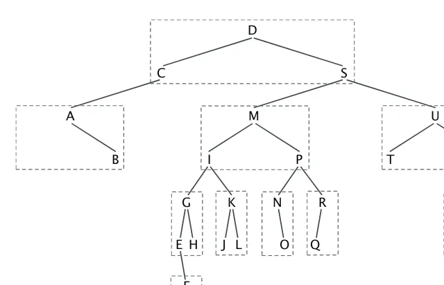
Our previous discussions suggest that there are many advantages to fixed-length records in terms of searching and file management, but they impose serious draw-backs in terms of efficient use of space. File indexing is an attempt to separate the issue of storage from the issue of access and management through the use of a sec-ondaryfile index. This allow us to use a fixed-lengthindex filefor managing and searching for records and a variable-lengthdata fileto store the actual contents of the records.
2.6.1 Simple Indices
We begin with a simple index: an array of key–offset pairs thatindexor report the location of a record with keykat offset positionpin the data file. Later, we will look at more complicated data structures like B-trees and external hash tables to manage indices more efficiently.
A key feature of an index is its support for indirection. We can rearrange records in the data file simply by rearranging the indices that references the records, without ever needing to touch the data file itself. This can often be more efficient; moreover, features like pinned records—records that are not allowed to change their position— are easily supported. Indices also allow us to access variable-length records through a fixed-length index, so we can support direct access to any record through its index entry’s offset.
TABLE 2.3
Indexing variable-length records: (a) index file; (b) data file
It’s also possible to store other (fixed-length) information in the index file. For example, since we are working with variable-length records, we might want to store each record’s length together with its key–offset pair.
2.6.2 Index Management
When an index file is used, changes to the data file require one or more corresponding updates to the index file. Normally, the index is stored as a separate file, loaded when the data file is opened, and written back, possibly in a new state, when the data file is closed.
For simple indices, we assume that the entire index fits in main memory. Of course, for large data files this is often not possible. We will look at more sophisti-cated approaches that maintain the index on disk later in the course.
Addition. When we add a new record to the data file, we either append it to the end of the file or insert it in an internal hole, if deletions are being tracked and if an appropriately sized hole exists. In either case, we also add the new record’s key and offset to the index. Each entry must be inserted in sorted key order, so shifting elements to open a space in the index, or resorting of the index, may be necessary. Since the index is held in main memory, this will be much less expensive than a disk-based reordering.
Deletion.Any of the deletion schemes previously described can be used to remove a record from the data file. The record’s key–offset pair must also be found and removed from the index file. Again, although this may not be particularly efficient, it is done in main memory.
to worry that the location of a deleted record might be moved to some new offset in the file.
Update.Updating either changes a record’s primary key, or it does not. In the latter case, nothing changes in the index. In the former case, the key in the record’s key– offset pair must be updated, and the index entry may need to be moved to maintain a proper sorted key order. It’s also possible in either case to handle an update with a deletion followed by an add.
2.6.3 Large Index Files
None of the operations on an index prevents us from storing it on disk rather than in memory. Performance will decrease dramatically if we do this, however. Multiple seeks will be needed to locate keys, even if we use a binary search. Reordering the index during addition or deletion will be prohibitively expensive. In these cases, we will most often switch to a different data structure to support indexing, for example, B-trees or external hash tables.
There is another significant advantage to simple indices. Not only can we index on a primary key, we can also index on secondary keys. This means we can provide multiple pathways, each optimized for a specific kind of search, into a single data file.
2.6.4 Secondary Key Index
Recall that secondary keys are not unique to each record; instead, they partition the records into groups or classes. When we build a secondary key index, its “offset” references are normally into the primary key index and not into the data file itself. This buffers the secondary index and minimizes the number of entries that need to be updated when the data file is modified.
ConsiderTable 2.4, which uses composer as a secondary key to partition music files by their composer. Notice that the reference for each entry is a primary key. To retrieve records by the composer Beethoven, we would first retrieve all primary keys for entries with the secondary key Beethoven, then use the primary key index to locate and retrieve the actual data records corresponding to Beethoven’s music files. Note that the secondary index is sorted first by secondary key, and within that by primary key reference. This order is required to support combination searches.
Addition.Secondary index addition is very similar to primary key index addition: a new entry must be added, in sorted order, to each secondary index.
Deletion.As with the primary key index, record deletion would normally require every secondary index to remove its reference to the deleted record and close any hole this creates in the index. Although this is done in main memory, it can still be expensive.
TABLE 2.4
A secondary key index on composer
secondary primary key
key reference
Beethoven ANG3795
Beethoven DGI39201
Beethoven DGI8807
Beethoven RCA2626
Corea WAR23699
Dvorak COL31809
· · ·
and subsequently reused, so if the secondary index were not updated, it would end up referencing space that pointed to new, out-of-date information.
If the secondary index references the primary key index, however, it is possible to simply remove the reference from the primary index, then stop. Any request for deleted records through the secondary index will generate a search on the primary index that fails. This informs the secondary index that the record it’s searching for no longer exists in the data file.
If this approach is adopted, at some point in the future the secondary index will need to be “cleaned up” by removing all entries that reference non-existent primary key values.
Update.During update, since the secondary index references through the primary key index, a certain amount of buffering is provided. There are three “types” of up-dates that a secondary index needs to consider.
1. The secondary key value is updated. When this happens, the secondary key index must update its corresponding entry, and possibly move it to maintain sorted order.
2. The primary key value is updated. In this situation, the secondary index must be searched to find the old primary key value and replace it with the new one. A small amount of sorting may also be necessary to maintain the proper by-reference within-key ordering.
3. Neither the primary nor the secondary key values are updated. Here, no changes are required to the secondary key index.
TABLE 2.5
Boolean
and
applied to secondary key indices for composer and
symphony to locate recordings of Beethoven’s Symphony #9
Beethoven Symphony #9 Result
ANG3795 ANG3795 ANG3795
DGI39201 COL31809
DGI8807 DGI8807 DGI8807
RCA2626
indices, then merging the results using Boolean operators to produce a final list of records to retrieve.
For example, suppose we wanted to find all recordings of Beethoven’s Symphony #9. Assuming we had secondary key indices for composer and symphony, we could use these indices to search for recordings by Beethoven, and symphonies named Symphony #9, thenandthese two lists to identify the target records we want ( Ta-ble 2.5).
Notice this is why secondary indices must be sorted by secondary key, andwithin
key by primary key reference. This allows us to rapidly walk the hit lists and merge common primary keys. Other types of Boolean logic likeor,not, and so on can also be applied.
2.6.5 Secondary Key Index Improvements
There are a number of issues related to secondary key indices stored as simple arrays:
• the array must be reordered for each addition, and
• the secondary key value is duplicated in many cases, wasting space.
If we use a different type of data structure to store the secondary key index, we can address these issues.
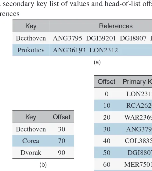
Inverted List.One possible alternative is to structure each entry in the secondary index as a secondary key value andnprimary key reference slots (Table 2.6a). Each time a new record with a given secondary key is added, we add the record’s primary key, in sorted order, to the set of references currently associated with that secondary key.
The advantage of this approach is that we only need to do a local reorganization of a (small) list of references when a new record is added. We also only need to store each secondary key value once.
TABLE 2.6
Alternative secondary index data structures: (a) an inverted list;
(b, c) a secondary key list of values and head-of-list o
ff
sets into a linked list
of references
Key References
Beethoven ANG3795 DGI39201 DGI8807 RCA2626
Prokofiev ANG36193 LON2312
(a)
Key Offset
Beethoven 30
Corea 70
Dvorak 90
(b)
Offset Primary Key Next
0 LON2312 ∅
10 RCA2626 ∅
20 WAR23699 ∅
30 ANG3795 80
40 COL38358 ∅
50 DGI8807 10
60 MER75016 ∅
70 COL31809 ∅
80 DGI39201 50
(c)
of choosing an array size: if it’s too small, the secondary key will fail due to lack of space, but if it’s too large, significant amounts of space may be wasted.
Linked List.An obvious solution to the size issue of inverted lists is to switch from an array of primary key references to a dynamically allocated linked list of refer-ences. Normally, we don’t create separate linked lists for each secondary key. In-stead, we build a single reference list file referenced by the secondary key index (Table 2.6b,c).3
Now, each secondary key entry holds an offset to the first primary key in the secondary key’s reference list. That primary key entry holds an offset to the next primary key in the reference list, and so on. This is similar to the availability list for deleted records in a data file.
There are a number of potential advantages to this linked list approach:
• we only need to update the secondary key index when a record is added,4or
when a record’s secondary key value is updated,
• the primary key reference list is entry sequenced, so it never needs to be sorted,
and
• the primary key reference list uses fixed-length records, so it is easy to
imple-ment deletion, and we can also use direct access to jump to any record in the list.
Sorting
FIGURE 3.1
Frozen raspberries are sorted by size prior to packaging
S
ORTING IS one of the fundamental operations will we study in this course. The need to sort data has been critical since the inception of computer science. For example, bubble sort, one of the original sorting algorithms, was analyzed to have average and worst case performance of On2in 1956. Although we know that comparison sorts theoretically cannot perform better than Onlgnin the best case, better performance is often possible—although not guaranteed—on real-world data. Because of this, new sorting algorithms continue to be proposed.We start with an overview of sorting collections of records that can be stored entirely in memory. These approaches form the foundation for sorting very large data collections that must remain on disk.
3.1
HEAPSORT
12 1 37
37
1 12
0
37
37 -9 12 -11
12 -5
12
FIGURE 3.2
A tournament sort used to identify the largest number in the
ini-tial collection
guarantees Onlgn performance, even in the worst case. In absolute terms, how-ever, heapsort is slower than Quicksort. If the possibility of a worst case On2is not acceptable, heapsort would normally be chosen over Quicksort.
Heapsort works in a manner similar to a tournament sort. In a tournament sort all pairs of values are compared and a “winner” is promoted to the next level of the tournament. Successive winners are compared and promoted until a single overall winner is found. Tournament sorting a set of numbers where the bigger number wins identifies the largest number in the collection (Figure 3.2). Once a winner is found, we reevaluate its winning path to promote a second winner, then a third winner, and so on until all the numbers are promoted, returning the collection in reverse sorted order.
It takes O ntime to build the initial tournament structure and promote the first element. Reevaluating a winning path requires O lgntime, since the height of the tournament tree is lgn. Promoting allnvalues therefore requires Onlgntime. The main drawback of tournament sort is that it needs about 2nspace to sort a collection of sizen.
Heapsort can sort in place in the original array. To begin, we define a heap as an arrayA[1. . .n] that satisfies the following rule.1
A[i]≥A[ 2i]
A[i]≥A[ 2i+1 ] )
if they exist (3.1)
To sort in place, heapsort splits Ainto two parts: a heap at the front ofA, and a partially sorted list at the end ofA. As elements are promoted to the front of the heap, they are swapped with the element at the end of the heap. This grows the sorted list and shrinks the heap until the entire collection is sorted. Specifically, heapsort executes the following steps.
1Note that heaps are indexed starting at 1, not at 0 like a C array. The heapsort algorithms will not
1. ManipulateAinto a heap.
2. SwapA[1]—the largest element inA—withA[n], creating a heap withn−1 elements and a partially sorted list with 1 element.
3. ReadjustA[1] as needed to ensureA[1. . .n−1] satisfy the heap property. 4. SwapA[1]—the second largest element inA—withA[n−1], creating a heap
withn−2 elements and a partially sorted list with 2 elements.
5. Continue readjusting and swapping until the heap is empty and the partially sorted list contains allnelements inA.
We first describe how to perform the third step: readjustingAto ensure it satisfies the heap property. Since we started with a valid heap, the only element that might be out of place is A[1]. The followingsift algorithm pushes an elementA[i] at positioniinto a valid position, while ensuring no other elements are moved in ways that violate the heap property (Figure 3.3b,c).
sift(A, i, n)
Input: A[ ], heap to correct;i, element possibly out of position;n, size of heap
while i ≤ ⌊n/2⌋ do
j = i*2 // j = 2i
k = j+1 // k = 2i + 1
if k ≤ nandA[k] ≥ A[j] then
lg = k // A[k] exists and A[k] ≥ A[j]
else
lg = j // A[k] doesn’t exist or A[j] > A[k]
end
if A[i] ≥ A[lg] then
return // A[i] ≥ larger of A[j], A[k]
end
swap A[i], A[lg] i = lg
end
So, to moveA[1] into place after swapping, we would callsift( A, 1, n-1 ). Notice thatsiftisn’t specific toA[1]. It can be used to move any element into place. This allows us to usesiftto convertAfrom its initial configuration into a heap.
heapify(A, n)
Input: A[ ], array to heapify;n, size of array
i = ⌊n/2⌋
while i ≥ 1 do
sift( A, i, n ) // Sift A[i] to satisfy heap constraints i−−
end
-5 12 8 0 21 1 -2
A[1] A[2] A[3] A[4] A[5] A[6] A[7] (a)
-5 12 8 0 21 1 -2
A[1] A[2] A[3] A[4] A[5] A[6] A[7] (b)
12 ↔ 21
-5 21 8 0 12 1 -2
A[1] A[2] A[3] A[4] A[5] A[6] A[7] (c)
21 12 8 0 -5 1 -2
A[1] A[2] A[3] A[4] A[5] A[6] A[7]
-5 ↔ 21 -5 ↔ 12
(d)
FIGURE 3.3
Heap construction: (a)
A
in its initial configuration; (b) sifting
A
[3] to confirm its position; (c) sifting
A
[2]
=
12 into place by swapping with
A
[5]
=
21; (d) sifting
A
[1]
=
−
5 into place by swapping with
A
[2]
=
21, then
with
A
[5]
=
12
After A[⌊n
2⌋] is “in place,” everything from A[⌊n
2⌋. . .n] satisfies the heap property. We move back to the element atA[⌊n2⌋ −1] and sift it into place. This continues until we siftA[1] into place. At this point,Ais a heap.
We use theheapifyandsiftfunctions to heapsort an arrayAas follows.
heapsort(A, n)
Input: A[ ], array to sort;n, size of array
heapify( A, n ) // Convert A into a heap
i = n
while i ≥ 2 do
swap A[ 1 ], A[ i ] // Move largest heap element to sorted list i−−
sift( A, 1, i ) // Sift A[1] to satisfy heap constraints
end

![FIGURE 3.3 Heap construction: (a) A in its initial configuration; (b) siftingA[3] to confirm its position; (c) sifting A[2] = 12 into place by swapping withA[5] = 21; (d) sifting A[1] = −5 into place by swapping with A[2] = 21, thenwith A[5] = 12](https://thumb-ap.123doks.com/thumbv2/123dok/3934747.1878167/51.612.67.375.68.334/construction-conguration-siftinga-conrm-position-swapping-swapping-thenwith.webp)